Functional Mode Analysis
We have developed a new technique called Functional Mode Analysis (FMA) that detects collective motions in biomolecules related to a specific function of the biomolecule. Given a large set to structures of one protein, for example from a molecular dynamics trajectory, the method detects a collective motion (or collective mode), that is maximally correlated to an arbitrary quantity of interest. In other words, the method aims to explain alterations in a quantity in terms of internal collective motions of the protein.
What kind of questions can be addressed with FMA?
Let us assume you are interested in a some ‘functional’ quantity that is important for the function of your protein, such as
- the volume of a binding site,
- the radius of gyration of the protein,
- the distance between two important functional residues,
- the number of H-bonds between two groups,
- the electrostatic potential at some site in the protein,
- etc,
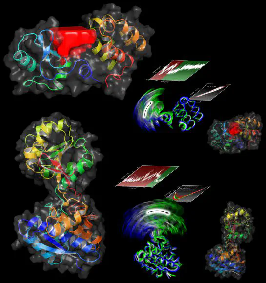
you may wonder how the protein accomplishes alterations of that quantity. FMA will detect the collective motion that is maximally correlated to your quantity and, hence, provide the link between protein function and collective motion. For instance, FMA demonstrates that substrate binding and release of T4 lysozyme are triggered by a hinge bending mode, whereas a twisting mode is required for the catalytic activity.
How is FMA related to normal mode analysis or principal component analysis?
Normal mode analysis (NMA) or principal component analysis (PCA) are popular techniques to identify the large-scale collective motions of proteins. NMA computes low-frequency modes and PCA yields the modes that give the largest contributions to the atomic RMSD in a given protein ensemble.
However, a functionally relevant mode is in most cases not identical to a specific normal or PCA mode, but may be distributed over a number of normal or PCA modes. For example, the electrostatic potential at a ligand binding site may be tuned by a combination of PCA vector no. 1, 3 and 15. In such cases, FMA yields a single collective mode which tunes the functional quantity. In addition, FMA quantifies the contributions of the individual PCA vectors (or normal modes) to the fluctuations of the functional quantity.
For more details on FMA, please check the original publication
In case you use results from FMA for a publication, we kindly ask you to cite the reference. Thank you!
Source code
Latest sources: fma.v0901.tar.gz
Please note that the software is distributed AS IS with NO WARRANTY OF ANY KIND, to the extent permitted by applicable law. The author is not responsible for any losses or damages suffered directly or indirectly from the use of the software. Use it at your own risk.
Releases
- v0.9. First release
- v0.901 (07/09/2009). Bug fix. FMA might have crashed when computing R as a function of number of eigenvectors.
Installation
There comes a README file with the source tar ball, which (hopefully) explains the compilation requirements and procedure. I have tested the installation under Mac OS X (10.5) and Suse Linux (Version 10), but for other environments the cmake input file might have to be further adapted (than explained in README). If you run into trouble, please do not hesitate to contact us (jochen dot hub at uni-saarland.de).
Please note: At present, the FMA code can only be linked to GROMACS 4.0.x. To compile and install GROMACS 4.07 on a Linux or Mac, you can use this script: install-gromacs4.07.sh. Please download the script, make it executable with chmod +x install-gromacs4.07.sh, and run it with ./install-gromacs4.07.sh. It will install GROMACS 4.07 in the current working directory. See the note in the script on how to use a specific compiler, if you don’t want ot use the default C/C++ compiler of your system. Important: This GROMACS 4.07 installation is not suitable for fast MD simulations because it does not use a fast FFT library. But it is fine to be used with FMA and to use the g_xxx GROMACS tools.
Problems, suggestions, bug reports
Please do not hesitate to send an email (jochen dot hub at uni-saarland.de) in case you run into trouble, have any suggestions, or if the documentation is unclear. Bug reports are also highly welcome.
Example (length of a helix)

If you are new with FMA, this example is probably where you want to start. The tar file contains a PDB structure of an alpha-helix, an GROMACS trajectory in XTC format, and a bash script with lots of comments and explanations. Note that his example is also shown in the supporting material of the FMA publication
The example demonstrates how to explain the changes in the length of a helix in terms of a collective motions of the helix. It also shows how to visualize the collective motions using, e.g., PyMol. This helix example does probably not provide striking new biological insight, but it useful for the user of FMA to get familiar with FMA in practice.
How-to-start tutorial
Please also check the fma help (including command line options) via fma -h.
The following instructions assume you use GROMACS. Let us assume you have the following input files:
A protein structure file
prot.pdb.A simulation trajectory in GROMACS xtc format,
traj.xtc.A data file observable with the functional variable $f(t)$. The file must have 2 columns, $time$ and $f(time)$.
Typically, you start with a PCA on the simulation
g_covar -s prot.pdb -f traj.xtc -v eigenvec.trrSelect the group for RMSD fit (typically backbone or C-alpha), and the group you want to use to explain the functional quantity (typically C-alpha, backbone, or heavy atoms).
Create the projections on the PCA vectors using
g_anaeigg_anaeig -s prot.pdb -f traj.xtc -v eigenvec.trr -proj proj.xvg -first 1 -last 50With option
-last, you choose the number of principal components (PCs) to write intoproj.xvg. Please note that the fma tool allows afterwords to choose (option-nvec) how many of the PCs inproj.xvgyou want to use in FMA. Unfortunately,g_anaeigwrites the projections in the awkward grace format with different PCs printed below each other, and separated by&characters. This format is horrible to parse, and the GROMACS-internal xvg read routine actually fails when parsing a really large xvg file. Therefore, please change the format using the bash scriptxvg2col.bashwhich is coming with the source code.xvg2col.bash proj.xvgThe script creates a file
proj.col.xvgwith one time column, followed by all the PC columns.Now, you can run the
fmatool. For the beginning, I suggest to stick the the Pearson coefficient as correlation measurefma -ip proj.col.xvg -i observable.xvg -iv eigenvec.trr -tmb ?? -ox -rc -rm -nev -contr -dvp ...The most important input options are
-tmb(final time for model builing): Time frames before-tmbwill be used for model building, time frame after-tmbfor cross validation-read-tmin,-read-tmax,-read-dt, defining first and last time to read, and the time step to read
Output: The output files are the following (xvg files are in grace format, use xmgrace to view). For the start, I suggest to check the output files r-crossv.xvg, r-modelbuild.xvg, and pear_nev.xvg. These plots allow to assess how successful FMA was in explaining the functional quantity in terms of a single functional mode.
r-crossv.xvg(option-rc): scatter plot (data vs. model) of the cross validation set, also providing the correlation $R_c$ between data and model of the cross validation building setr-modelbuild.xvg(option-rm): scatter plot (data vs. model) of the model building set, also providing $R_m$, i.e. the correlation between data and model in the model building setpear_nev.xvg(option-nev): $R_c$ and $R_m$ as a function of the number of PCA vectors d used as basis set. Likewise,sig_nev.xvg(option-nevs) provides the standard deviation between data and model as a function of d. That output is important to find a reasonable number of PCA vectors that are used as basis set to construct the collective mode.validate.xvg(option-od) plots the functional quantity, the model in the model building set, and the model in the validation set as a function of time.linmodel.xvg(option-lm): parameters $β_i$ of the linear model (compare publication). The subtitle of the plot provides the equation how to compute the functional quantityf from the projection $p_a$ on the functional mode.collvec.xvg(option-ox): parameters $α_i$ of the functional mode a (the maximally correlated motion) with respect to the PCA vectors.contr.xvg(option-contr): contributions of different principal components (PCs) to the variance of the model. In addition, the plot shows the variance of the PCs, i.e. the PCA eigenvalues if the same frames were used for PCA and FMA. (The values $(β_iσ_i)^2$ are rather for test issues).dataVsPa.xvg(option-dvp): data f versus the projection $p_a$ on the functional mode.MCM.trr(option-va): Cartesian atomic coordinates of the maximally correlated motion (the vector a in the publication). Can be further used withg_anaeig2(see below)ewMCM.trr(option-vew): Cartesian atomic coordinates of the ensemble-weighted maximally correlated motion (ewMCM). Can be further used withg_anaeig2(see below).
Visualization of collective modes MCM and ewMCM
You can use the g_anaeig2 -extr option to create movies of the maximally correlated motion (MCM) or the ensemble-weighted MCM (ewMCM). Example videos of such motions are available as supporting material of the FMA publication (see here, for example). To visualize the extreme extensions along the MCM in your trajectory, use something like
g_anaeig -s prot.pdb -f traj.xtc -v MCM.trr -extr mcm-extr.pdb -nframes 30
Note that since the MCM written in MCM.trr is normalized, the spacial displacement visible in mcm-extr.pdb may appear smaller than in the simulation (and depends on the number of basis vectors used in FMA, option -nvec). Therefore, you may want to use the -max option of g_anaeig to visualize the MCM.
To visualize the ewMCM, you can use the g_anaeig command lines that fma prints to the console (check fma output). The motion that makes the functional quantity $f$ fluctuate within $n \cdot \sigma f$ (where $\sigma f$ is the standard deviation of $f$) is generated by
g_anaeig -s prot.pdb -v ewMCM.trr -max n -extr ewMCM.pdb -nframes 30
To get a good impression of the motion, you may want to choose $n = 3$. Alternatively, if you want to visualize the motion that generates the extremes of $f$, you can use the g_anaeig2 tool that comes with the FMA implementation. The only difference between g_anaeig2 and the normal g_anaeig is that it provides a -min option in addition to the -max. (Hopefully the official g_anaeig will soon provide the -min option.) Use arguments for -min and -max are in the fma output. The command line may be similar to:
g_anaeig2 -s prot.pdb -v ewMCM.trr -min -8.25553 -max 7.68362 -extr ewMCM.pdb -nframes 30
Finally, the motions in mcm-extr.pdb or ewMCM.pdb may be visualized with common visualization software (such as PyMol).
Frequently Asked Questions (FAQ)
While compiling, I am getting an error message such as
/usr/bin/ld: cannot find -lf2c, what’s wrong?
Answer: Either you don’t have thef2clibraries installed (try locatelibf2c, if you have locate on your system), or you have not adapted the lineset (LIBDIR_F2C /sw/lib)in the
CMakeLists.txtfile.While compiling I get link errors such as
undefined reference to `sgesv_'Answer: The compiler does not find the LAPACK/BLAS libraries.
Make sure that- the path to the LAPACK/BLAS libs is correctly given inin
set(LAPACKDIR /home/me/path_to_lapack)CMakeLists.txt, - the names of the LAPACK/BLAS libs is given byDepending on the file names, that line may also read
set (LIBLAPACK lapack blas)orset (LIBLAPACK lapack_LINUX blas_LINUX)or similar.set (LIBLAPACK lapack_APPLE blas_APPLE)
Important: The names must be given without thelibat the beginning of the file name. - And that the LAPACK/BLAS library file names on your hard disk start with
lib. If the LAPACK/BLAS libs are called (e.g.)lapack.aandblas.a, please use themvcommand to rename them toliblapack.aandlibblas.a.
- the path to the LAPACK/BLAS libs is correctly given in
While compiling, I get link errors such as
undefined reference to `for_len_trim'
undefined reference to `for_write_seq_fmt'
undefined reference to `for_write_seq_fmt_xmit'
undefined reference to `for_stop_core'
What’s wrong?
Answer: Please try against link to the gfortran libraries, that may help. Please change the lineset (LIBS m md_mpi gmx_mpi f2c ${LIBLAPACK})to
set (LIBS m md_mpi gmx_mpi gfortran f2c ${LIBLAPACK})in
CMakeLists.txt.Installing f2c on a Fedora Linux. If you are having trouble installing
f2con a Fedora system, this website may help you.
Any suggestions? I am happy to add them here.