Practical 12: Free energy calculations

A. The free energy “slow-growth” method

Molecular simulations can be carried out to gain either dynamic or energetic information on the simulated system. Today we’ll focus on different ways to extract energies and free energies from simulations. One way to gain access to free energies by simulation is to perform so-called free-energy perturbation (FEP) or thermodynamic integration (TI) simulations. In such simulations, the system is gradually “morphed” from one state to another (let’s say from state “A” to state “B”), during which the effect of this perturbation on the free energy is monitored. In practice, this is achieved by defining a morph parameter lambda, which is defined to be zero in the initial state (A), and one in the final state (B). By collecting the derivative of the potential energy concerning lambda during the simulation, and by integrating over lambda afterward, we gain access to the free energy.

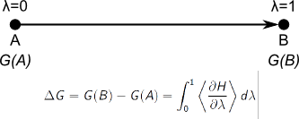
Note that, in case that the masses (and hence the kinetic energies) do not depend on λ, dH/dλ reduces to dV/dλ, as used in the lecture.

B. Solvation-free energy of a sodium ion in water

We are now going to use this procedure to calculate the free energy of solvation for a sodium ion in water. For this, we’ll slowly create a sodium ion in a water box. In order to start the simulation, download the starting coordinates, the topology, and the MD parameter file first. Let’s have a look at the starting structure:

pymol start.pdb

To show a simulation box, in PyMol window type:

show cell
show spheres, resn NA

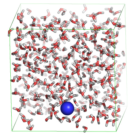
Note that the sodium ion is already “present” in the starting structure. Now have a look at the topology na.top, with xedit, nedit, more or less, and look for the line containing Na under [ atoms ]. You’ll notice that two states (A and B) are defined, with charges 0 and 1, respectively. This means that during the simulation, the charge of the sodium ion will be slowly switched on.

Now start the simulation:

source /home/gromacs/softwarerc
gmx grompp -f fep -c start.pdb -p na
gmx mdrun -v -c charged.gro

Analyze the free energy change by:

xmgrace dhdl.xvg

To compute the free energy, we must integrate dH/dλ over dλ. Instead, we have dH/dλ as a function of time. This is not a problem, as we know that lambda changed from 0 to 1 during this time (10 ps). So instead, we can integrate the curve over time, and divide the obtained value by ten to derive the desired free energy. To integrate, under Data, select Transformations, followed by Integration, and press Accept.

Question: The experimentally observed solvation-free energies for sodium range from -365 to -372 kJ/mol. How does the obtained value correspond to that?

Instead of integrating dH/dλ, we can also compare the initial and final values of the potential energy of the system:

gmx energy

Select Potential, followed by 0 (and, if necessary, an extra “enter”).

xmgrace energy.xvg

Subtract the initial value from the final value.

Question: What value do you get? Why is this value different from the free energy difference obtained by integrating dH/dλ?

One important check in simulations in general and free energy simulations, in particular, is to make sure that the answer has converged. To do so, we can either perform a longer (or shorter!) simulation, and compare the result to the original, or we can perform the backward transition to see if the free energy difference is the opposite of the forward transition. In this practical, we’ll do both. First, we’ll carry out the backward transition. Copy the MD parameter file to incorporate the changes:

cp fep.mdp back.mdp

Open back.mdp in your favorite editor (xedit, nedit, emacs, kate, vi) to make the following changes:

First search for Free energy, then change init-lambda to 1 and change delta-lambda to -0.0002. Now we can start the backward simulation. For this, we’ll use the final structure of the previous simulation (charged.gro) as the initial structure:

gmx grompp -f back -c charged.gro -p na -maxwarn 2
gmx mdrun -v

And analyze the free energy change using xmgrace. Remember that we now changed lambda from zero to one, meaning that if we integrate over time, we should divide the obtained value by -10 instead of by 10.

Question: What value do you get? How does this value compare to the free energy change for the forward simulation? Would you consider the obtained value for the solvation-free energy sufficiently converged?

Question: If we take the forward and backward simulation together, is the total free energy change positive or negative? Which of the two should it have been?

As stated above, another way to check convergence is to perform a longer simulation and see if the free energy change remains the same as compared to a shorter simulation. For this, open fep.mdp in your favorite editor. Change nsteps from 5000 to 50000, and delta-lambda from 0.0002 to 0.00002, and repeat the forward transition:

gmx grompp -f fep -c start.pdb -p na
gmx mdrun -v

This time divide the integration result in xmgrace by 100.

Question: Is the obtained free energy very different as compared to the shorter simulations? What would you consider an appropriate length for this type of simulation?

C. Thermodynamics of reversible peptide folding

For the case of a sodium ion in water, we could compute the free energy difference between two states because we defined a path connecting the two states, and we had access to the free energy gradient along the path. In the case of the ion in water, the path was artificial (hence such free energy perturbation studies are also called “computational alchemy”). Likewise, a free energy difference can also be computed along a real path, e.g. by forcing an ion across an electrostatic gradient and integrating the force required to displace the ion along the path.

There are also cases, however, where such a path, artificial or real, can not be easily defined. Peptide or protein folding is a good example. The problem of defining a path is that there are multiple folding (and unfolding) pathways that connect the (well-defined) folded state and the degenerate unfolded state. If we would like to compute the folding free energy by integrating the force along a pathway connecting the two, we’d therefore have to follow multiple pathways and take a weighted average of the results. In the case, however, where we have a simulation in which folding and unfolding take place spontaneously (i.e. without forcing the system to fold or unfold) and reversibly we can also access the free energy difference between the folded and unfolded state in a different way, namely simply by monitoring the fraction of time the system resides in each state. In the equilibrium case (i.e. if the simulation was long enough to visit all relevant configurations multiple times) the probability of finding the system is exactly proportional to its Boltzmann factor. Therefore, for any two states, the following equation holds:

$$ \frac{p_1}{p_2} = e^{- \frac{\Delta G}{k_B T}} $$

with $\Delta G = G_1 - G_2$

Therefore, if we know the respective probability of finding the system in a particular pair of states, we can calculate the free energy difference between these two states. Note that for this type of free energy calculation, we solely need the conformational information (coordinates, trajectory) from the simulation, no energies!

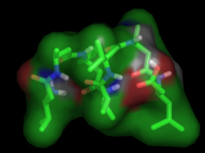
To illustrate the above, we are going to calculate the free energy of the folding of a small peptide. For this, download a PDB file of the peptide and the MD trajectories at four different temperatures: 298K, 340K, 350K and 360K.

First view part of one trajectory with VMD:

gmx trjconv -s pep.pdb -f 340.xtc -o movie.pdb -e 10000 -fit rot+trans

and select 4 followed by 1 when asked to select a group.

vmd movie.pdb

In VMD, play with different representations (under Graphics → Representations, e.g. Licorice and then in tab Trajectory → Trajectory Smoothing Window Size to about 10) and press the “play” button on the bottom of the main window. You see the first folding transition during the simulation at 340 K.

Question: What kind of structure is the folded structure?

For a more quantitative analysis of the folding/unfolding transitions, we’ll analyze the root mean square deviation of each structure in each trajectory with respect to the folded structure. Here we will call the structure “folded” if it has a root mean square deviation (RMSD) of less than 2 Angstroms (0.2 nm) of the backbone atoms with respect to the reference structure in pep.pdb.

gmx rms -s pep.pdb -f 340.xtc -o rmsd_340.xvg

When asked for a selection of groups, press “4” (Backbone) and “4” (Backbone) again. View the result with xmgrace:

xmgrace rmsd_340.xvg

Question: How many folding/unfolding transitions do you observe?

Repeat the same procedure for the other 3 temperatures to generate rmsd_298.xvg, rmsd_350.xvg and rmsd_360.xvg. With a command like the following, we can count how many configurations from each trajectory are “folded” or “unfolded”:

cat rmsd_340.xvg | awk 'NR >13 &&$2 < 0.2 {print $0}' | wc -l

ONLY in case this didn’t work, you can try with the next command. See explanation below:

cat rmsd_340.xvg | sed 's/0\./0,/g' | awk ' NR > 13 && $2 < 0.2 {print $0}' | wc -l

(never mind if you didn’t understand that command completely. We first throw away the header of the rmsd_340.xvg file, and afterward awk only prints the lines of which the second column (the RMSD) is smaller than 0.2; the wc -l simply counts the number of lines). The sed command, finally, replaces the dots in the file with commas, for the case your computer expects German input, which uses commas for floating point numbers. The obtained number is the number of “folded” configurations in the 340K simulation. Repeat the procedure, now to count the number of “unfolded” conformations. You’ll see, at this temperature, the system is folded about one-third of the time.

Question: What about the other three temperatures? What would you estimate to be the folding temperature?

Question: Do the above free energy estimates, based on peptide configurations, include the influence of the solvent? Would different folding-free energies (and/or an estimate of the folding temperature) be obtained when the solvent is analyzed as well?

Question: Assuming that the folding enthalpy is the same for the different temperatures, how can the entropy difference between the folded and unfolded state be estimated from the set of free energies? How large do you estimate the entropy of folding in this case? Is it positive or negative? Why?

Hope you enjoyed it. In case of questions or suggestions, please do not hesitate to contact us.

Further references

Books

• Editors: Chipot C., Christophe A. et al., Free Energy Calculations Springer Series in Chemical Physics, Vol. 86, [link].

Advanced reading

• R. W. Zwanzig, High Temperature Equation of State by a Perturbation Method. I. Nonpolar Gases J. Chem. Phys. 22: 1420 (1954). [link]
• Goette M, Grubmuller H, Accuracy and convergence of free energy differences calculated from nonequilibrium switching processes J. Comp. Chem. 30: 447-456 (2009). [link]