A. Introduction
In the previous lecture, we learned about the importance of long-range electrostatic interactions for an accurate modeling of biomolecular macromolecules in aqueous solution. Today’s practical will deal with the computation of these interactions using the so-called non-linear Poisson-Boltzmann equation (PBE) introduced during the last lecture. $$ \nabla \cdot \left [ \epsilon(\mathbf{r}) \nabla \phi(\mathbf{r}) \right ] = \rho_{\text{macro}}(\mathbf{r}) + \sum_{i} q_i n_{i}^{0} e^{\frac{-q_i \phi(\mathbf{r})}{k_B T}} $$
In the equation above $n_{i}^{0}$ is the number density of ions of type $i$ in the bulk solution, $q_i$ is the charge on the ion, $\phi(\mathbf{r})$ is the electrostatic potential in that region of space, $k_B$ is Boltzmann’s constant and $T$ is the temperature. $\rho_{\text{macro}}(\mathbf{r})$ is the charge density due to the macromolecule under consideration. Note that the dielectric constant $\epsilon(\mathbf{r})$ is a function of the location in $R^3$ (inhomogeneous $\epsilon(x,y,z)$). The nonlinear PBE given above can be linearized via a Taylor expansion of the sum at the right-hand side (as shown in the lecture).
To obtain solutions of the PBE on a computer, we are going to use APBS (Adaptive Poisson-Boltzmann Solver), a software package for evaluating the electrostatic properties of nanoscale biomolecular systems, which is already installed on the computers you are working with. APBS solves the Poisson-Boltzmann equation numerically by means of a finite difference/finite element approach.
The files needed for this practical can be downloaded here. To download and extract directly in the terminal use:
wget https://biophys.uni-saarland.de/storage/courses/pract/p8/PBE_prakt.tar.gz
tar xzvf PBE_prakt.tar.gz
📚 Refreshing your memory with some important concepts
Polarizability
Polarizability refers to the ability of a molecule or a material to form instantaneous or induced dipoles when subjected to an external electric field. In simpler terms, it measures how easily the electron cloud within an atom or molecule can be distorted by an external electric field.
Types of polarization
- Electronic polarization: Here when the external field is applied, the electron clouds of the atoms are displaced with respect to the heavy nuclei within the dimensions of the atoms.
- Ionic polarization: It occurs only in some ionic crystals. In the presence of an external electric field, the positive and negative ions are displaced up to the point where ionic bonding forces stop this displacement. Hence dipoles get induced.
- Orientational polarization: It applies only to polar dielectric materials. Generally, in the absence of an external electric field, electric dipoles are oriented randomly; having a zero polarizability net effect. However, in the presence of an electric field, these dipoles try to rotate and align in the direction of the electric field.
Dielectric Constant (Relative Permittivity)
The dielectric constant, often denoted by the symbol ε (epsilon), is a measure of a material’s ability to store electrical energy in an electric field. It’s a dimensionless quantity that represents how much the electric field within the material is reduced compared to the electric field in a vacuum.
Relationship between polarizability and dielectric constant
The relationship between polarizability and dielectric constant is typically seen in the context of how the polarizability of atoms or molecules within a material affects the material’s overall dielectric constant. It’s particularly important in understanding the behavior of materials in capacitors and dielectric media.
High Polarizability: Materials with high polarizability tend to have higher dielectric constants. This is because they can easily form and sustain induced dipoles when exposed to an electric field, which enhances their ability to store electrical energy.
Low Polarizability: Materials with low polarizability have lower dielectric constants. They are less capable of forming induced dipoles and storing electrical energy in an electric field.
In summary, polarizability influences how readily a material responds to an electric field, while the dielectric constant reflects the material’s ability to store electrical energy. The relationship between them lies in how the polarizability of individual atoms or molecules contributes to the overall dielectric behavior of the material.
B. Simple example: Born solvation
The Generalized Born (GB) equation is an approximation of the PBE. It models atoms as charged spheres whose internal dielectric is lower than that of the environment.
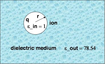
As a first and rather straightforward step we are computing the solvation-free energy of an ion with charge $q$ and radius $a$ (or $r$ in the previous picture) embedded in a dielectric continuum with dielectric constants $\epsilon_{\text{out}}$. The ion itself has a dielectric constant of $\epsilon_{\text{in}}$. In other words, $\epsilon_{\text{in}}$ and $\epsilon_{\text{out}}$ denote the internal and external (solution) dielectric constants, respectively. If $\epsilon_{\text{in}}$ is chosen to be 1, the result obtained is the free energy change associated with transferring an ion from the gas phase into a solution with dielectric constant $\epsilon_{\text{out}}$. In our Born solvation model, we assume zero ionic strength.
$$ \Delta_p G_{\text{Born}} = \frac{q^2}{8 \pi \epsilon_0 a} \left ( \frac{1}{\epsilon_{\text{out}}} - \frac{1}{\epsilon_{\text{in}}} \right ) $$
Two things are needed to run a calculation with APBS:
- An input file for APBS and
- A so-called PQR file, which is an augmented PDB file that also contains the partial charge and the radius of the respective atom in the occupancy and temperature columns, respectively.
On the cip-pool computers you first need to instruct the shell where to look for the APBS:
export PATH=$PATH:/home/gromacs/apbs/apbs/build/bin
Change to the directory born. Then run APBS:
cd PBE_prakt/born
apbs apbs.in
For our Born solvation model, the PQR file only contains one atom with a partial charge +1. It looks like this:
REMARK  This is an ion with a 3 A radius and a +1 e charge
REMARK  located at position (0.,0.,0.)
ATOM      1   I  ION     1 0.000   0.000   0.000  1.00 3.00
The input file for APBS is somewhat more extended and looks like this:
# READ IN MOLECULES
read
    mol pqr born.pqr       # Read molecule 1
end

# CALCULATE POTENTIAL FOR SOLVATED STATE
elec name solvated
    mg-manual
    dime 65 65 65
    nlev 4
    grid 0.33 0.33 0.33
    gcent mol 1
    mol 1
    lpbe
    bcfl mdh
    pdie 1.0                # Solute dielectric
    sdie 78.54              # Solvent dielectric
    chgm spl2
    srfm mol
    srad 1.4
    swin 0.3
    sdens 10.0
    temp 298.15
    gamma 0.105
    calcenergy total
    calcforce no
    write pot dx pot
end

# CALCULATE POTENTIAL FOR REFERENCE STATE
elec name reference
    mg-manual
    dime 65 65 65
    nlev 4
    grid 0.33 0.33 0.33
    gcent mol 1
    mol 1
    lpbe
    bcfl mdh
    pdie 1.0
    sdie 1.0                  # Solvent dielectric
    chgm spl2
    srfm mol
    srad 1.4
    swin 0.3
    sdens 10.0
    temp 298.15
    gamma 0.105
    calcenergy total
    calcforce no
end

# COMBINE TO FORM SOLVATION ENERGY
print energy solvated - reference
end

# SO LONG
quit
First, APBS reads the PQR file named born.pqr. Then two PBE calculations with different solvent dielectric constants, 1 and 78.54 will be carried out.
Question: Why are we using these values?
The two groups are named solvated and reference, and the difference between these two free energies will be printed at the end of the run.
The other parameters in the input file are not important for this practical, but you can find more details here.
# READ IN MOLECULES
read
  mol pqr born.pqr
end
elec name solv # Electrostatics calculation on the solvated state mg-manual # Specify the mode for APBS to run
dime 97 97 97 # The grid dimensions
nlev 4 # Multigrid level parameter
grid 0.33 0.33 0.33 # Grid spacing
gcent mol 1 # Center the grid on molecule 1
mol 1 # Perform the calculation on molecule 1
lpbe # Solve the linearized Poisson-Boltzmann equation
bcfl mdh # Use all multipole moments when calculating the potential pdie 1.0 # Solute dielectric
sdie 78.54 # Solvent dielectric
chgm spl2 # Spline-based discretization of the delta functions
srfm mol # Molecular surface definition
srad 1.4 # Solvent probe radius (for molecular surface)
swin 0.3 # Solvent surface spline window (not used here)
sdens 10.0 # Sphere density for accessibility object
temp 298.15 # Temperature
calcenergy total # Calculate energies
calcforce no # Do not calculate forces
end
Compare your computed result with the analytical value obtained via
$$ \Delta_p G_{\text{Born}} = -\frac{691.85 \text{ kJ/mol Å}}{R} $$
Where $R$ is the radius of the ion.
We can now also display the electrostatic potential by typing
source /home/gromacs/softwarerc
vmd -e pot_field.vmd
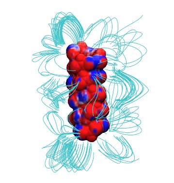
C. Electrostatic potential of the ion channel Gramicidin A
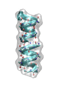
Now we are ready to perform a PBE calculation on a biomolecular macromolecule. To this end, we have chosen the ion channel Gramicidin A (gA) in its helical form. Gramicidin A is a derivative of gramicidin, an antibiotic consisting of a heterogeneous mixture of six antibiotic compounds. Gramicidin A is a linear polypeptide containing 15 amino acids. It kills pathogenic organisms by destroying the cationic (Na+, K+, H+) concentration gradients over the bacterial membrane, which are vital for their proper functioning. In other words, monovalent cations can easily leak through gA once they are incorporated into the cell membrane of the organism.
Have a look at the structure of the helical gA dimer by typing (first change into the correct folder).
cd ../gA
vmd -e gA.vmd
and rotating the polypeptide. Also, have a look at the SYSTEM.pqr file.
Question: What is so far the (only) major difference compared to the previous Born ion example?
At this point, we need to specify the internal (i.e. inside the protein) dielectric constant for our calculation (remember: in the Born solvation case the internal dielectric constant was set to 1). With the dielectric constant being a macroscopic observable, but the biomolecular macromolecule being a nano-sized molecular entity, it is often not clear what value to choose, and one should consider the internal dielectric constant as an adjustable parameter within the PBE framework. It usually ranges from 2 to 20, depending on the molecular details of the macromolecule under consideration.
Question: What determines the lower bound of the range for bimolecules? Are bimolecules polarizable?
We can now easily perform the PBE calculation inside VMD. VMD - Visual Molecular Dynamics - is a molecular visualization program for displaying, animating, and analyzing large biomolecular systems using 3-D graphics and built-in scripting. You need to highlight the START.pdb representation in the Main window, right mouse click and choose Load data into molecule. Then choose SYSTEM.pqr and click Load. This will load the PQR file for gA. Now go to the Extensions section in the VMD Main window and select Analysis → APBS Electrostatics. Click on Edit (the one between Add and Delete) and change the number of the x, y and z grid points from 129 to 65. Also, change the solute (protein) dielectric constant from 1.0 to 10. Press OK and start the PBE calculation by pressing Run APBS.
You can follow the APBS computation in the “vmd console” window. After completion accept to load the electrostatic potential into the top molecule. APBS calculation should be completed in a few seconds.
In case APBS calculations take more time, stop the calculation by pressing ctr + c in the VMD terminal.
Then, load the already generated APBS output file pot.dx. You need to highlight the START.pdb representation in the Main window, right mouse click and choose Load data into molecule. Then choose pot.dx and click Load. This will load the pot.dx file for gA.
One can map the electrostatic potential onto a generated molecular surface by creating a new representation changing the drawing method to Surf, coloring method to Volume and setting the probe radius to 1.1 Angstrom. Then in Trajectory adjust the Color Scale Data Range to -1 and 1, respectively. We can check on the sign of the potential by inspecting the coloring scheme used in the representation. To do so we go to Graphics → Color - Color Scale. In addition, the color scale bar can be shown by Extensions → Visualization → Color Scale Bar. Adjust the maximum and minimum in the Color Scale Bar window to 1 and -1 respectively. Now you can zoom into the channel region. The striking feature is that the channel area as well as the entrance area show the same coloring, which means the sign of the potential is the same. If VMD is not functioning properly you can download the snapshots of the electrostatic potential isosurfaces. In the terminal use
wget https://biophys.uni-saarland.de/storage/courses/pract/p8/gA_snapshots.tar
Or just download; then
tar xvf gA_snapshots.tar
Question: What sign of the potential would you expect for a cation-selective channel (i.e. a channel that permeates positively charged ions)?
D. Ion permeation free energy profile for Gramicidin A
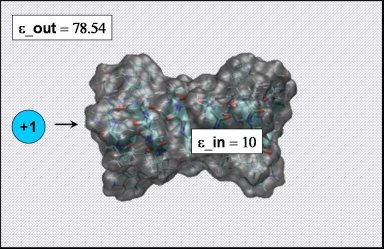
To compute the free energy profile for cation migration through gA using the PBE we only need to add one cation to an existing PQR file of gA and repeat the calculations from the previous example for varying ion positions. To speed up the process, there are already 9 PQR files with equidistant ion positions spanning the range from -16.0 to +16.0 Å in your working directory. Please have a look at one of the SYSTEM.pqr.* files first. (To do this go to the directory gA_ions cd ../gA_ion/).
ATOM    547  HA2 ETA    17       2.016 -10.455  -4.104  0.090 1.320
ATOM    548  CB  ETA    17       2.566 -12.311  -5.091  0.050 2.175
ATOM    549  HB1 ETA    17       2.983 -13.305  -4.818  0.090 1.320
ATOM    550  HB2 ETA    17       1.624 -12.457  -5.663  0.090 1.320
ATOM    551  OG  ETA    17       3.493 -11.626  -5.922 -0.660 1.770
ATOM    552  HG1 ETA    17       3.762 -12.236  -6.614  0.430 0.224
ATOM    553  Na  ION     3      -2.675  16.000  -1.764  1.000 1.908
END
We can also have a look at the sequence of differing ion positions inside gA by typing
vmd -e snapshots.vmd
As in the Born solvation example, we also need to compute a reference state that only contains the cation embedded in pure water ( those coordinates can be found in the ion.pqr.* files: have a look at one of them). If we subtract the two computed free energies we get the difference in free energy between the cation being solvated by pure water and the cation being solvated at a fixed position by gA, which is hydrated by water (Note that we are only interested in the free energy difference, so no complete thermodynamic cycle needs to be computed!). The working directory contains a script that will perform the 9 independent pairs of PBE calculations and write the total free energy into a file named total_energy. The APBS parameters are given in apbs.in.
Question: What protein dielectric constant is initially used?
You can now start the script by typing
./PBE_loop
For each snapshot shown the script will run a PBE calculation and extract the solvation-free energy difference (you will have to eventually merge it into the respective cation position). After the calculation is finished, you can plot the free energy profile using e.g. gnuplot
gnuplot
plot "total_energy" w lp
plot "total_energy" u :1 smooth csplines w lp
Question: Why should the profile be symmetric? Why is it not the case?
You can press exit to escape from the gnuplot session.
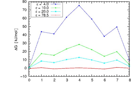
You can now change the solute dielectric constant in the apbs.in the file, repeat the previous computation cycle and try to reproduce the plot shown below, using different values of epsilon.
Hint
💡 In case you find it too tedious to change the dielectric constants by hand and to keep track of the file names, you may use the script diel_serie.sh found in the gA_ion directly. Such scripts are extremely useful for automating calculations, avoiding errors, ensuring results reproducibility, and documenting what you have done. Take a look at the script (e.g. with emacs), and try to understand what it does. Then run:
./diel_serie.sh
and look at the output with
xmgrace -legend load total_energy_*_normalised
The graph illustrates the dependence of the free energy profile as a function of the protein dielectric constant. The free energy barrier for Na+ migration through gA is estimated to be ~ 50 kJ/mol.
Question: Which dielectric constant will give a result close to the experiment? Which dielectric constant would you choose if there were no experimental values to compare with?
Question: What can we learn from this plot? Does it have the correct asymptotic behavior as epsilon_in approaches 78.54?
Question: An alternative would be to estimate the free energy profile from MD simulations of the gramicidin channel embedded in a lipid bilayer membrane surrounded by water. In such MD simulations, the dielectric constant is usually set to 1. How do you expect that choice to affect the result? To answer this, recall what kind of polarization is well represented in standard MD simulations, and what kind of polarization is not represented.
Further references
Acknowledgment
This practical is largely based on a practical by Udo W. Schmitt.