Practical 03: Introduction to protein structure

A. Introduction

In the last lectures, we learned how protein structures are determined experimentally. Today, we’ll focus on how computational techniques are employed to aid structure determination.

There are three main techniques for solving protein structures: x-ray crystallography, Nuclear Magnetic Resonance (NMR), and cryo-electron microscopy (cryo-EM). As can be seen from the current Protein Data Bank (PDB) holdings on Wikipedia, or on the PDB site, roughly 160,000 protein structures have been solved so far, and are all available for download from the Protein Data Bank. About 8% of these are NMR structures, 3% are cryo-EM structures, and the rest are x-ray crystallographic structures. As can also be seen on the PDB holdings list, the number of solved proteins grows constantly, due to advancements in structure determination techniques. Nevertheless, the number of known protein sequences is orders of magnitude larger (currently about 180,700,000, as available from the UniProtKB/Swiss-Prot database).

B. Reading PDB files

Experimentally solved protein structures are stored at the Protein Data Bank, from which individual protein structures can be retrieved as so-called PDB files. Before we turn to the structure determination itself, let us have a closer look at a typical PDB file, to see what can be learned about the background of the structure (experimental conditions, etc.) and the structural quality (the resolution, coordinate uncertainty, etc). We will focus on PDB entry 1DWR (an x-ray structure of myoglobin-carbon monoxide complex) as it can be downloaded from the Protein Data Bank.

PDB file format

The initial lines of a PDB entry contain information on:

• The protein, date of deposition, and PDB ID code.
• The biological source of the macromolecule.
• List of authors who sent the entry to the PDB.
• References to the literature that describe the structure in detail.
• Some basic information regarding the crystallographic data.

Especially critical to check are the resolution, the R-factor and free-R factor, which contain information on how well the deposited structure matches the measured data (x-ray reflection intensities in this case). Here, the former two metrics are explained in detail.

HEADER    OXYGEN TRANSPORT                        11-DEC-99   1DWR              
TITLE     MYOGLOBIN (HORSE HEART) WILD-TYPE COMPLEXED WITH CO                   
COMPND    MOL_ID: 1;                                                            
COMPND   2 MOLECULE: MYOGLOBIN;                                                 
COMPND   3 CHAIN: A                                                             
SOURCE    MOL_ID: 1;                                                            
SOURCE   2 ORGANISM_SCIENTIFIC: EQUUS CABALLUS;                                 
SOURCE   3 ORGANISM_COMMON: HORSE;                                              
SOURCE   4 ORGANISM_TAXID: 9796;                                                
SOURCE   5 ORGAN: HEART                                                         
KEYWDS    OXYGEN TRANSPORT, RESPIRATORY PROTEIN                                 
EXPDTA    X-RAY DIFFRACTION                                                     
AUTHOR    K.CHU,J.VOJTECHOVSKY,B.H.MCMAHON,R.M.SWEET,J.BERENDZEN,               
AUTHOR   2 I.SCHLICHTING                                                        
REVDAT   3   24-FEB-09 1DWR    1       VERSN                                    
REVDAT   2   29-APR-05 1DWR    1       REMARK HET    HETNAM FORMUL              
REVDAT   2 2                           HETATM                                   
REVDAT   1   03-MAR-00 1DWR    0                                                
JRNL        AUTH   K.CHU,J.VOJTECHOVSKY,B.H.MCMAHON,R.M.SWEET,                  
JRNL        AUTH 2 J.BERENDZEN,I.SCHLICHTING                                    
JRNL        TITL   CRYSTAL STRUCTURE OF A NEW LIGAND BINDING                    
JRNL        TITL 2 INTERMEDIATE IN WILDTYPE CARBONMONOXY MYOGLOBIN              
JRNL        REF    NATURE                        V. 403   921 2000              
JRNL        REFN                   ISSN 0028-0836                               
JRNL        PMID   10706294                                                     
JRNL        DOI    10.1038/35002641                              
[..] 
REMARK   2                                                                      
REMARK   2 RESOLUTION.    1.45 ANGSTROMS.                                       
REMARK   3                                                                      
REMARK   3 REFINEMENT.                                                          
REMARK   3   PROGRAM     : X-PLOR 3.851                                         
REMARK   3   AUTHORS     : BRUNGER                                              
REMARK   3                                                                      
REMARK   3  DATA USED IN REFINEMENT.                                            
REMARK   3   RESOLUTION RANGE HIGH (ANGSTROMS) : 1.45                           
REMARK   3   RESOLUTION RANGE LOW  (ANGSTROMS) : 20                             
REMARK   3   DATA CUTOFF            (SIGMA(F)) : 0.0                            
REMARK   3   DATA CUTOFF HIGH         (ABS(F)) : NULL                           
REMARK   3   DATA CUTOFF LOW          (ABS(F)) : NULL                           
REMARK   3   COMPLETENESS (WORKING+TEST)   (%) : 96.1                           
REMARK   3   NUMBER OF REFLECTIONS             : 23794               
REMARK   3  
REMARK   3  FIT TO DATA USED IN REFINEMENT.                                     
REMARK   3   CROSS-VALIDATION METHOD          : THROUGHOUT                      
REMARK   3   FREE R VALUE TEST SET SELECTION  : RANDOM                          
REMARK   3   R VALUE            (WORKING SET) : 0.211                           
REMARK   3   FREE R VALUE                     : 0.255                           
REMARK   3   FREE R VALUE TEST SET SIZE   (%) : 5.0                             
REMARK   3   FREE R VALUE TEST SET COUNT      : NULL                            
REMARK   3   ESTIMATED ERROR OF FREE R VALUE  : NULL                       
[..]
REMARK   3  RMS DEVIATIONS FROM IDEAL VALUES.                                   
REMARK   3   BOND LENGTHS                 (A) : 0.013                           
REMARK   3   BOND ANGLES            (DEGREES) : 1.93                            

C. X-ray crystallography

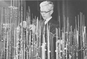
The main technique for determining protein structures is x-ray crystallography. Since the first protein structure (myoglobin) was solved by this technique by John Kendrew and Max Perutz in the late 1950s, several thousand others followed. As can be appreciated from the picture on the right, which shows John Kendrew with the structural model of myoglobin, at that time the determination of a structure with the size of a protein, without the aid of a computer, was a formidable task.

It is important to note that in both x-ray crystallography and NMR, protein structures are not measured directly in the experiment. Rather, a set of data is collected (a diffraction pattern or an NMR spectrum), from which a model of the protein structure is derived. To appreciate the difference between data and structure, we’ll now look at two different structures of the same protein, and the corresponding x-ray crystallographic data. For this, we will concentrate on the bacterial light-driven proton pump bacteriorhodopsin (bR). Click here for more background information on bR.

First download two bR structures from the Protein Data Bank, with PDB entries 1BRR and 1QHJ. Save both PDB files to your local account (see the last practical if you forgot how to download from the PDB). View the structures with PyMol:

pymol 1BRR.pdb 1QHJ.pdb

Align both structures with 1BRR→(A)→align→to molecule (*/CA)→1QHJ.

To focus only on one of the protein’s chain, types (in the PyMol prompt):

select A, chain A and polymer
hide all
show cartoon, A

Feel free to play with the color. Click in the right menu, e.g. (A)→C→spectrum→rainbow. Try to show as lines or sticks selection A. Hide and show the structures to check for differences.

To highlight the dye (the light sensor in the protein interior), create a new atom selection, and show it in licorice representation:

select retinal, resn RET

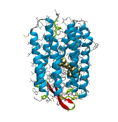
Then click (A)→S→licorice (or spheres).

Question: By looking at the structures and the PDB entry, which of the two structures would you prefer, in terms of coordinate accuracy?

Remember, so far we only looked at the coordinates, which represent a model that was optimized against the measured data. So, let us now have a look at the data. In X-ray crystallography, data are collected by measuring a diffraction pattern that is obtained from x-rays reflected by a protein crystal. As mentioned in the lecture, this diffraction pattern itself does not suffice to determine the complete structure since only the amplitudes of the diffracted waves were collected, not their phases. In X-ray crystallography, however, there are several tricks available to obtain phases (e.g. isomorphous replacement, molecular replacement), but we will not go into that in detail here. What is important to remember is that eventually, an atomic electron density map is obtained.

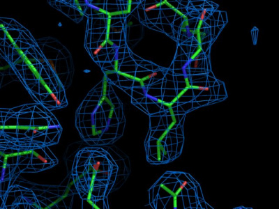
Visit the Protein Data Bank in Europe (PDBe) to view the electron density map of 1BRR. Enter the PDB code (1BRR), wait for the search result to appear, and click the 1brr entry. Several plots with information on this structure are available. Feel free to browse around to check the meaning of the individual plots. In the menu to the right, choose 3D Visualization. By clicking atoms (and waiting for a few seconds), electron densities should be visualized. For instance, you could click on one of the retinals, and see the density as a blue transparent surface.

Try to get a bit familiar with the viewer (mouse wheel, hold left or right mouse bottom, SHIFT+mouse wheel to change clipping and fog).

To visualize the electron density, three types of maps are useful based on: the observed diffraction data (Fo) and the diffraction data calculated from the atomic model (Fc).

• 2Fo-Fc is an “all features” map, which is the best way to calculate an estimate of the true electron density from diffraction data and atomic model. (It is called 2Fo-Fc because the calculation involves combining the observed diffraction data, Fo, with the diffraction data calculated from the atomic model, Fc, in a way that gives the least-biased result). Typically contoured at 1 sigma, it shows how well the observed density fits around the atomic mode
• Fo-Fc is a “difference map”. It shows where the experimental density and the atomic model disagree
  • +ve, observed higher than the atomic model.
  • -ve, observed lower than the atomic model.

Different isosurfaces are controlled with the $\sigma$ parameter.

As you move the mouse over the backbone trace of the protein, individual residues are highlighted in pink, and the residue number is highlighted at the bottom right of the window. Click a residue around residue number 80, and inspect the electron density. For instance, take a close look at Tyr-79, which contains a six-membered aromatic ring. Do you find the electron density for the aromatic ring convincing? Optionally, play with the isosurface levels by adjusting the 2Fo-Fc σ value in the Map menu on the right.

Move to one of the loops that connect the transmembrane helices. Click one of them, and inspect the electron density.

Repeat the procedure for entry 1QHJ.

Question: What is the agreement between the structural model and electron density here, for aromatic groups, loops, and retinal?

Question: Based on the data and the model structures, would you say there is a large impact of the resolution of the data on the accuracy of the structural model?

The highest resolution x-ray crystallographic structures could have rounds the 0.8 Å or even somewhat better. To see an example of such a dataset, look at the density for structure 2B97. In the viewer, first show individual atoms and color them by element (Polymer→...→Add Representation→Ball & Sticks and delete the former representation below in the menu; Polymer→Set Coloring→Element Symbol). Now take a look at the electron density, do you notice the difference?

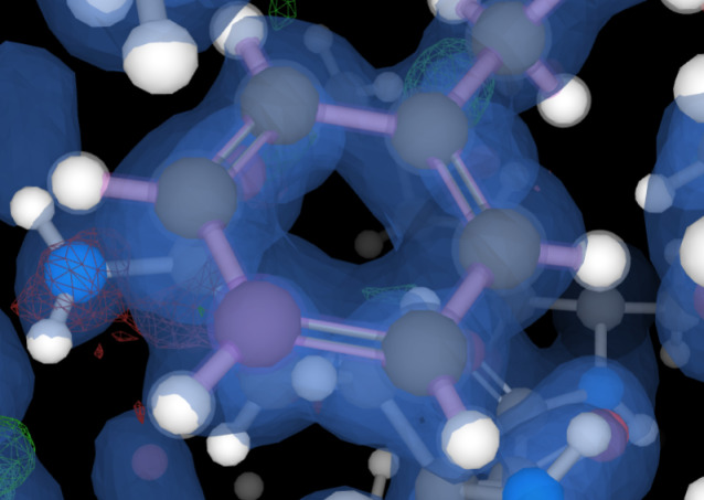
Question: Can you discuss whether observing hydrogen atoms, such as those in the aromatic Phe-8 residue, is feasible using the electron density isosurface? Play with the electron density isosurface (move the bar at Volume Streaming→2Fo-Fc with your mouse). Why are hydrogen atoms still difficult to see, even at such high resolution?

A measure for the coordinate uncertainty of the individual atoms due to the thermal motion in the crystal is given by the temperature factor (or B factor). Low B-factors (< 30) correspond to well-defined parts of the structure, whereas high B-factors (> 80) might indicate highly disordered parts of the structure or even misinterpreted parts of the model.

D. NMR

The other main technique for determining protein structures is NMR. In contrast to x-ray crystallography, no crystals are required for an NMR experiment. Rather, the structure is determined by the protein in solution. Therefore, it has the advantage that the protein can be studied in its native environment. On the other hand, the resolution of an NMR structure is usually lower and there is a size limitation of a few hundred amino acids for structure determination using NMR.

It would go beyond the scope of this course to explain the NMR experiment in detail. We will therefore only briefly touch on the experimental setup and then focus on the structure building and refinement step based on the obtained data. The NMR signal is recorded as a nuclear magnetic resonance spectrum of predominantly the hydrogen atoms after the sample has been subjected to a (number of) strong magnetic pulse(s). Mainly hydrogen atoms give rise to the signal, because of the magnetic spin properties of the hydrogen nucleus (a proton). The naturally occurring isotopes of the other elements that are found in proteins, carbon (¹²C) and oxygen (¹⁶O), have a zero nuclear magnetic moment. Nitrogen (¹⁴N) does have a non-zero magnetic moment, but can usually not be used in NMR, for reasons that would go beyond the scope of this course to explain. These elements, therefore, can only be utilized in NMR experiments when chemically replaced by a specific isotope, like ¹³C or ¹⁵N. The most structurally relevant information is usually obtained from a so-called NOESY experiment (Nuclear Overhauser Enhancement Spectroscopy). The Nuclear Overhauser Effect or Nuclear Overhauser Enhancement is the change (enhancement) of the signal intensity from a given nucleus as a result of exciting or saturating the resonance frequency of another nucleus. Since this effect is distance-dependent, it can be used to derive the distance between an interacting pair of protons. In practice, protons closer than 6 Å apart can be identified this way.

Now, we will calculate a model of the structure of a small protein, the B1 domain of protein G, from the proton-proton distance information obtained from a NOESY experiment. Download the data file containing the distance information here. You can have a look at the file (with the program more or less or a browser or editor of your choice) to assure yourself that there are indeed only distance bounds listed in this file. Additionally, we need an initial guess of the structure. Since we don’t know the structure yet, we have to start from an unstructured peptide chain, which can be obtained here. Have a look at the structure with:

pymol proteinG.pdb

Finally, we need something called a molecular topology, a chemical description of the protein: which atoms the molecule contains, which atoms are covalently bonded to each other, etc. This molecular topology file is available here. Now, in principle, we have all the data to attempt to build a structure that is in agreement with all experimentally determined distances. The only thing we still need is an input file for the CNS program.

Note that, in contrast to x-ray crystallography, where a single structure is presented, to reflect the fact that the NMR experiment probes an ensemble of protein molecules in solution, an NMR structure is usually represented by an ensemble of structures, that all fulfill the NMR data. To run CNS, we need to add to the environmental variable PATH an extra library called libg2c and the version corresponding to our architecture:

export LD_LIBRARY_PATH=/home/gromacs/cns/libg2c
export PATH=$PATH:/home/gromacs/cns/cns_1.1/intel-i686-linux/bin:/home/gromacs/cns/cns_1.1/intel-i686-linux/utils

Then, start CNS with

tcsh
source /home/gromacs/cns/cns_1.1/cns_solve_env

If you get an error try to source it again. This might solve the problem.

cns < anneal.inp

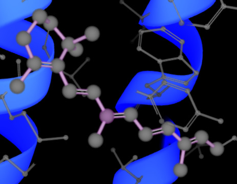
10 structures of the B1 domain of protein G will now be calculated by simulated annealing. This is a computationally intensive calculation, as the structure is slowly, dynamically transformed from the extended starting conformation to the real structure, by a slow-cooling simulation, also called simulated annealing. As the calculation is running, we can have a look at how exactly such a calculation proceeds, and how the final structure is generated from the starting guess. Download this file, open another shell, and open the just downloaded file in PyMol:

pymol sa.pdb

In the PyMol prompt, type:

show wire

Then press the play button at the bottom right of the main PyMol window, to see an animation of the simulated annealing structure calculation procedure. If the movie plays too fast, on the menu, under movie→speed, choose a different speed.

When the CNS structure calculation has finished, switch back to that window. You can now close the tcsh session with ctr + d. Then type:

cat anneala_*.pdb > anneal.pdb

To combine all ten generated structures into one file. View the result with:

pymol anneal.pdb

Question: Which parts of the structure are well-defined, and which parts show more ambiguity?

There is also an x-ray structure available of the B1 domain of protein G, available under the PDB code 1PGB. Download it from the Protein Data Bank and compare it to the just calculated NMR structure. Hint: within PyMol, use the commands:

fetch 1PGB
align 1PGB, anneal_0001
zoom

Question: What are the main differences between the NMR and x-ray structures of the B1 domain of protein G?

E. Optional

• Change the initial temperature of the annealing simulation in the file anneal.inp.
• Change the final temperature of the annealing simulation in the file anneal.inp.

Question: How do you anticipate that adjusting these parameters will impact the simulation results?

Further references

Principles of protein structure and basic in biophysics and biochemistry

• Kessel and Ben-Tal, Introduction to Proteins: Structure, Function and Motion
• Cantor and Schimmel, Biophysical Chemistry Part I: The conformation of biological macromolecules
• PDB website tutorial
• Electron density maps

Advanced reading:

• K Henzler-Wildman and D Kern. Dynamic personalities of proteins, Nature 450: 964-972 (2007). [link]