Practical 02: Introduction to protein simulation

A. Introduction

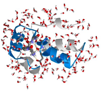
In the previous part, we’ve learned what MD simulations are and how to simulate a Van-der-Waals gas. Now it is time to set up a simulation of a biological macromolecule: a small protein.

Proteins are nature’s universal machines. For example, they are used as building blocks (e.g. collagen in skin, bones and teeth), transporters (e.g. hemoglobin as oxygen transporter in the blood), reaction catalysts (enzymes like lysozyme that catalyze the breakdown of sugars), and nano-machines (like myosin that is at the basis of muscle contraction). The protein’s structure or molecular architecture is sufficient for some of these functions (like for example in the case of collagen), but for most others, the function is intimately linked to internal dynamics. In these cases, evolution has optimized and fine-tuned the protein to exhibit exactly that type of dynamics that is essential for its function. Therefore, if we want to understand protein function, we often first need to understand its dynamics (see references below).

Unfortunately, there are no experimental techniques available to study protein dynamics at the atomic resolution at the physiologically relevant time resolution (that can range from seconds or milliseconds down to nanoseconds or even picoseconds). Therefore, computer simulations are employed to numerically simulate protein dynamics.

As before, we will use the GROMACS simulation package for this.

Today, we will simulate the dynamics of a small, typical protein domain: the B1 domain of protein G. B1 is one of the domains of protein G, a member of an important class of proteins, which form IgG binding receptors on the surface of certain Staphylococcal and Streptococcal strains. These proteins allow the pathogenic bacterium to evade the host immune response by coating the invading bacteria with host antibodies, thereby contributing significantly to the pathogenicity of these bacteria (click here for further background information on this protein).

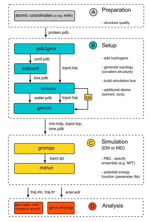
We will now follow a standard protocol to run a typical MD simulation of a protein in a box of water in gromacs. The individual steps are summarized in a flowchart on the right site.

B. How to do the practical from home

Mount your Cip Pool directories by the set-up alias as explained in Moodle or:

mkdir -p ~/mnt/cip-home
sshfs UNI_ID@gordon.cip.physik.uni-saarland.de:/home/UNI_ID ~/mnt/cip-home -o auto_cache,reconnect

Where UNI_ID is your university account id (s8…) and navigate to there (cd ~/mnt/cip-home). Create and enter the directory for today (e.g. mkdir pract2; cd pract2) In another terminal get to your Cip Computer - again through an established alias or changing the 207

ssh -t -XC UNI_ID@gordon.cip.physik.uni-saarland.de "ssh -t -XC 134.96.87.207"

C. Preparation

GROMACS commands are done in the directory on the Cip machine, visualization (VMD, PyMol or xmgrace) on yours. Before a simulation can be started, an initial structure of the protein is required. Fortunately, the structure of the B1 domain of protein G has been solved experimentally, both by x-ray crystallography and NMR. Experimentally solved protein structures are collected and distributed by the Protein Data Bank (PDB). Please open this link in a new browser window and enter “protein G B1” in the search field. Several entries in the PDB should match this query. We will choose the x-ray structure with a high resolution (entry 1PGB with a resolution of 1.92 Å) for this study. To download the structure, click on the link “1PGB”, and then, under “Download Files”, select “PDB File”. When prompted, select “save to disk”, and save the file to the local hard disk (click here if that does not work). To have a look at the contents of the file, on the Unix prompt, type:

less 1PGB.pdb

Next, get the software needed for the practical into your path:

source /home/gromacs/softwarerc

or for the VirtualBox:

source /home/gromacs/gromacs-5.15/bin/GMXRC.bash

As we’ll learn in the next practical on protein structure, the file starts with general information about the protein, about the structure, and about the experimental techniques used to determine the structure, as well as literature references where the structure is described in detail. (in less, use page up/page down/arrow up/arrow down to scroll). The data file contains the atomic coordinates of our protein structure with one line per atom. (quit the less program by pressing q). Now we can have a look at the structure:

pymol 1PGB.pdb

To visualize the structure. We now see the protein in cartoon representation (showing the secondary structure), as well as some water atoms as little crosses. To show all protein atoms, click (in the menu on the right) S → wire (Show wireframe representation) (some PyMOL versions don’t have wire representation and you can use sticks). Note that atoms (with different colors for the different chemical elements: green for carbon; red for oxygen and blue for nitrogen) are not shown directly, but the bonds between atoms are shown as lines. Under S, also try other representations such as sticks, spheres, surface and cartoon. To hide a representation, use the H button next to the S button. Exit PyMol with the cross at the top right of the window, or use Ctrl-C in the Linux shell.

D. Setup

We will now prepare the protein structure to be simulated in GROMACS. Although we now have a starting structure for our protein, one might have noticed that hydrogen atoms (which would appear white) are still missing from the structure. This is because hydrogen atoms contain too few electrons to be observed by X-ray crystallography at moderate resolutions. Also, GROMACS requires a molecular description (the “topology”) of the molecules to be simulated before we can start, containing information on e.g. which atoms are covalently bonded and other physical information. Both the generation of hydrogen atoms and the writing of the topology can be done with the GROMACS program pdb2gmx:

gmx pdb2gmx -f 1PGB.pdb -o conf.pdb

when prompted for the force field to be used, choose the number corresponding to the OPLS-AA/L all-atom force field, and SPC/E for water. View the result with:

pymol conf.pdb

See the added hydrogens, after clicking S → wire The topology file written by pdb2gmx is called topol.top. Have a look at the contents of the file using:

less topol.top

you will see a list of all the atoms (with masses, and charges), followed by bonds (covalent bonds connecting the atoms), angles, dihedral angles etc. Near the very end of the topology (in the [ molecules ] section) there is a summary of the simulation system, including the protein and 24 crystallographic water molecules. The topology file thus contains all the physical information about all interactions between the atoms of the protein (bonds, angles, torsion angles, Lennard-Jones interactions and electrostatic interactions).

The next step in setting up the simulation system is to solvate the protein in a water box, to mimic a physiological environment. For that, we first need to define a simulation box. In this case, we will generate a rectangular box with the box edges at least 7 Angstroms apart from the protein surface:

gmx editconf -f conf.pdb -o box.pdb -d 0.7

(note that GROMACS uses units of nanometers). View the result with

pymol box.pdb

and, in the PyMol prompt, type:

show cell

Now, exit PyMol and fill the simulation box with SPC water using the solvate module:

gmx solvate -cp box.pdb -cs spc216 -o water.pdb -p topol.top

Again, view the output (water.pdb) with PyMol. Now the simulation system is almost ready. Before we can start the dynamics, we must perform an energy minimization.

For the energy minimization, we need a parameter file, specifying which type of minimization should be carried out, the number of steps, etc. For your convenience, a file called em.mdp has already been prepared and can be downloaded from here. View the file with less to see its contents. We use the GROMACS preprocessor to prepare our energy minimization:

gmx grompp -f em.mdp -c water.pdb -p topol.top -o em.tpr

This collects all the information from em.mdp, the coordinates from water.pdb and the topology from topol.top, checks if the contents are consistent and writes a unified output file: em.tpr, which will be used to carry out the minimization:

gmx mdrun -v -s em.tpr -c em.pdb

The output shows that already the initial energy was rather low, so in this case, there were hardly any bad contacts. Having a look at em.pdb shows that the structure hardly changed during minimization.

The careful user may have noticed that grompp gave a warning:

System has non-zero total charge: -4.

Before we continue with the dynamics, we should neutralize this net charge of the simulation system. This is to prevent artifacts that would arise as a side effect caused by the periodic boundary conditions used in the simulation. A net charge would result in electrostatic repulsion between neighboring periodic images. Therefore, 4 sodium ions will be added to the system:

gmx genion -s em.tpr -o ions.pdb -np 4 -p topol.top

Select the water group (SOL), and 4 water molecules will be replaced by sodium ions. The output (ions.pdb) can be checked with PyMol. To better see the ions, type (in PyMol):

select Na, resn NA

A new group Na is now listed in the menu on the right. Show the new group Na as spheres, and choose a new color via the C button, next to the S and H buttons.

E. Simulation

Just to be on the safe side, we repeat the energy minimization, now with the ions included. Remember to (re)run grompp to create a new run input file whenever changes to the topology, or coordinates have been made. Before rerunning grompp and mdrun, let us delete some files to make sure new and old files are not confused:

rm -f em.tpr em.pdb traj_comp.xtc
gmx grompp -f em.mdp -c ions.pdb -p topol.top -o em.tpr
gmx mdrun -v -s em.tpr -c em.pdb

Now we have all that is required to start the dynamics. Again, a parameter file has been prepared for the simulation, and can be downloaded here. Please browse through the file md.mdp (using less) to get an idea of the simulation parameters. The GROMACS online manual describes all parameters in detail here. Please don’t worry in this stage about all individual parameters, we’ve chosen common values typical for protein simulations. Again, we use the GROMACS preprocessor to prepare the simulation:

gmx grompp -f md.mdp -c em.pdb -p topol.top -o md.tpr

and start the simulation!

gmx mdrun -v -s md.tpr -c md.pdb

The simulation is running now, and depending on the speed and load of the computer, the simulation will run for some minutes.

F. Analysis of a GROMACS simulation

The simulation is running now (or finished) and we can start analyzing the results. Let us first see which kind of files have been written by the simulation (mdrun):

ls -lrt

That shows the newest files at the bottom of the output. We see the following files:

• traj_comp.xtc - the (compressed) trajectory to be used for analyses
• traj.trr - the trajectory in full precision, which is normally not needed
• ener.edr - energies computed during the simulation
• md.log - a LOG file of mdrun
• md.pdb - the final coordinates of the simulation

The first analysis step during or after a simulation is usually a visual inspection of the trajectory. For this, we will use the GROMACS trajectory viewer VMD or PyMOL.

Before we visualize the trajectory, we make sure that molecules in the trajectory file are not broken over the periodic boundaries:

gmx trjconv -s md.tpr -f traj_comp.xtc -pbc mol -o whole.xtc

And choose 0 (System) when asked for the output group.

vmd em.pdb whole.xtc

Press the Play button in the main VMD window. You can also move the progress bar left and right with the mouse, and change the speed at which the movie is played. To represent protein and solvent differently, go to Graphics → Representations. In the Representations window, you can create two different representations (Button Create Rep), and enter protein or water into the Selected Atoms box, respectively. Try different ways to visualize protein and water in the Drawing Method drop-down menu (such as New Cartoon, VDW, CPK, or Licorice). With a double-click on the representation groups, you can turn the groups on and off. You can also play with the color, highlighting atoms by the element, amino acid type (polar, apolar, charged, …), etc. A three-dimensional impression of the protein, supported by an intuitive visual representation, often helps to understand the function of a protein.

An alternative visualization is provided by PyMol. First, we have to extract the protein coordinates and write in PDB format:

gmx trjconv -s md.tpr -f whole.xtc -o traj.pdb -dt 1

Now, select group 1 (Protein). And view with PyMol:

pymol traj.pdb

On the PyMol prompt, type:

dss

followed by

show wire

In addition, click the S (show), H (hide), and C (color) bottoms on the right top panel and play with possible representations and colors. Holding the right, left, or middle mouse button while moving the mouse allows you to rotate, zoom, and move the protein. Play the animation by pressing the play button. For a more quantitative analysis of the protein fluctuations, we can view how fast and how far the protein deviates from the starting (experimental) structure:

gmx rms -s md.tpr -f traj_comp.xtc

When prompted for groups to be analyzed, type 1 1. g_rms has written a file called rmsd.xvg, which can be viewed with:

xmgrace rmsd.xvg

We see the Root Mean Square Deviation (RMSD) from the starting structure, averaged over all protein atoms, as a function of time.

If we now wish to see if the fluctuations are equally distributed over the protein, or if some residues are more flexible than others, we can type:

gmx rmsf -s md.tpr -f traj_comp.xtc -oq -res

Select group 3 (C-alpha). The result can be viewed with:

xmgrace rmsf.xvg &

We can see that four regions in the protein show large flexibility: around residues 1, 11, 21 and 38. To see where these residues are located in the protein, type:

pymol bfac.pdb

Type spectrum b into the PyMol prompt. The protein backbone is now shown with the flexibility color-encoded. The red (orange, yellow) regions are relatively flexible and the blue and green regions are relatively rigid.

The simulation not only yields information on the structural properties of the simulation but also on the energetics. With the program gmx energy the energies written by mdrun can be analyzed:

gmx energy -f ener.edr

Select Potential and end your selection by pressing enter twice, View the result with:

xmgrace energy.xvg

As can be seen, the total potential energy initially rises rapidly after which it relaxes again. (To see the initial rise, you may need to zoom into the data points at t=0, using the magnifier/zoom tool of xmgrace (🔍). Click the AS button to return to the original zoom.)

Please repeat the energy analysis for several different energy terms to obtain an impression of their behaviors.

Question: Do you think the length of our simulation is sufficient to provide a faithful picture of the protein’s conformations at equilibrium?

We continue with several more specific analyses, the first of which is an analysis of the secondary structure (alpha-helix, beta-sheet) of the protein during the simulation.

First, we need to tell GROMACS where the DSSP program for secondary structure calculations can be found:

export DSSP=/home/gromacs/dssp/dssp

(or, if you get a message export: Command not found., you’re perhaps using a (t)csh in which case the command should be setenv DSSP /usr/global/whatif/dssp/dssp)

Now, perform the actual analysis with:

gmx do_dssp -s md.tpr -f traj_comp.xtc -ver 2

select group 1 (protein), and convert the output to PostScript with:

gmx xpm2ps -f ss.xpm

and view the result with:

gv plot.eps

As can be seen, the secondary structure is rather stable during the simulation, which is an important validation check of the simulation procedure (and force field) used. The next thing to analyze is the change in the overall size (or gyration radius) of the protein:

gmx gyrate -s md.tpr -f traj_comp.xtc

(again, select group 1 for the protein)

xmgrace gyrate.xvg

The analysis shows that the gyration radius fluctuates around a stable value and does not show any significant drift. Another important check concerns the behavior of the protein surface. To this end, we compute the hydrophobic and the hydrophilic solvent-accessible surface area (SASA):

gmx sasa -s md.tpr -f traj_comp.xtc -surface 'group "Protein"' -output '"Hydrophobic" group "Protein" and charge {-0.15 to 0.15}; "Hydrophilic" group "Protein" and not charge {-0.15 to 0.15}'

Now view the solvent-accessible surface area with:

xmgrace -nxy area.xvg

We now see three curves together: black for the total accessible surface, green for the hydrophilic accessible surface, and red for the hydrophobic accessible surface.

Question: Is the total (solvent-accessible) surface constant? Are any hydrophobic groups exposed during the simulation?

G. Optional

• You’ve probably noticed that in the simulation only around ten percent of the system that was simulated consisted of protein, the rest was water. As we are mainly interested in the protein’s motions and not so much in the surrounding water, one could ask if we couldn’t forget about the water and rather simulate the protein. That way, we could reach ten times longer simulations with the same computational effort!

  Question: Why do you think that it is important to include explicit solvent in the simulation of a protein?

  💡 To check if your assumption is correct, repeat the simulation of protein G, this time without solvent. To observe the effect more clearly, increase the length of the simulation by changing < in the file md.mdp by e.g. a factor of ten.

  Question: What are the main differences to the protein’s structure and dynamics as compared to the solvent simulation?

  💡 Use programs like gmx rms and gmx gyrate to analyze both simulations

• Let’s go back to the first step in setting up the system - as we already know, building the topology of our protein can be done with the GROMACS program pdb2gmx:

  gmx pdb2gmx -f 1PGB.pdb -o conf_gromos.pdb
  

  When prompted for the force field to be used, choose the GROMOS 43a1 instead of OPLS-AA/L. Use less and rasmol commands as before to compare the result with the previous configuration - what difference do you find?

  Question: How is the level of representation correlated with system size (number of atoms)?

Further references

Principles of protein structure and basic in biophysics and biochemistry

• Stryer, Biochemistry
• Kessel and Ben-Tal, Introduction to Proteins: Structure, Function and Motion
• Cantor and Schimmel, Biophysical Chemistry Part I: The conformation of biological macromolecules

Computer simulations and molecular dynamics

• M. Karplus and A. McCammon. Molecular Dynamics simulations of biomolecules, Nature structural biology 9: 646-652 (2002). [link]
• D.C. Rapaport. The Art of Molecular Dynamics Simulations - 2nd edn, Cambridge University Press (2004).

Advanced reading

• H. Scheraga, M. Khalili and A. Liwo. Protein-Folding Dynamics: Overview of Molecular Simulation Techniques, Annual Review of Physical Chemistry 58: 57-83 (2007).[link]
• K Henzler-Wildman and D Kern. Dynamic personalities of proteins, Nature 450: 964-972 (2007). [link]
• K A Sharp and B Honig. Electrostatic Interactions in Macromolecules: Theory and Applications, Annual Review of Biophysics and Biophysical Chemistry 19: 301-332 (1990).
• F M Richards. Areas, Volumes, Packing, and Protein Structure, Annual Review of Biophysics and Bioengineering 6: 151-176 (1977).
• K A Dill, S B Ozkan, M Scott Shell and T R Weikl. The Protein Folding, Problem Annual Review of Biophysics 37: 289-316 (2008).