Practical 01: Introduction to molecular dynamics simulations: simulation of argon

A. Introduction

Often it is necessary to understand the dynamics of a biomolecule in order to understand its function. For proteins, much information can usually be derived from the structure, or even based solely on the sequence, but the detailed functional mechanism often includes a structural transition or atomic fluctuations of the protein or substrate that can only be understood if the underlying atomistic dynamics are known in detail. The functional dynamics of proteins typically take place on a picosecond to millisecond timescale. Unfortunately, there are hardly any experimental techniques available with a high enough time and spatial resolution to follow the atomistic motions step by step, to be able to view proteins “in action”, like under a microscope. Therefore, computer simulations of the atomic motions are the methods of choice to study biomolecular dynamics. Such simulations allow insights into the dynamics involved in e.g. enzyme catalysis, molecular motors, molecular transport, or molecular recognition, in atomic detail. Today we will learn how to set up such a so-called molecular dynamics simulation, first on a simple system (argon gas), after which we will turn to a real protein.

B. MD simulation of argon

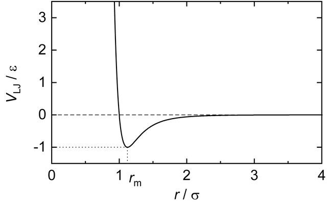
As a first case study, we consider the dynamics of Argon gas. Argon is a noble gas, characterized by a high degree of inertness (i.e. it is chemically relatively unreactive). Physically, it is a relatively simple compound, as it is mono-atomic both as gas and as fluid (no covalent bonds that form molecules) and because it is apolar. Therefore, it can be modeled as a neutral compound. Concerning the “force-field”, as it has been introduced during the lectures, it means that in argon the only relevant force-field terms are the Pauli-repulsion (that prevent atoms from overlapping) and London-dispersion (induced dipole-dipole interactions), which together are described by a Lennard-Jones potential. Hence, in simulation jargon, Argon and other noble gases are also referred to as Lennard-Jones fluids.

The simulations will be carried out with the GROMACS simulation package. On the GROMACS homepage, you can find both the software and documentation (online reference and paper manual). To run a simulation, three input files are usually required:

• A structure file: contains the atomic coordinates of the system to be simulated
• A “molecular topology”: contains the atomic simulation parameters (force-field) and a description of the bonds, bond angles (if any), Lennard-Jones parameters etc. of the simulation system
• The simulation parameters: type of simulation, number of steps, simulation temperature, etc.

C. Condensation and boiling of Argon

Let’s start by moving to your home directory (your own user directory) with the cd command. Without a parameter, this command brings you to your home directory. Now let’s create a directory for our first simulation of argon at 100K and change the directory with:

mkdir argon_100K
cd argon_100K

For the Argon simulations, three files have already been prepared. Download argon_start.pdb, argon.top and md.mdp to your local working directory without changing the filenames. Please feel free to have a look at these files (on the command prompt, you can open these files with any of the following programs: more, less, xedit, emacs, vi, kate).

Gromacs is used with the command gmx followed by the name of a GROMACS module and further command line options. To get gmx (and some other software) into your path, run the following command in the Linux terminal:

source /home/gromacs/softwarerc

GROMACS uses the preprocessor grompp to collect the data from the three input files, checks the internal consistency, and writes one unified input file, topol.tpr On the command prompt in a Linux terminal or shell, type:

gmx grompp -f md.mdp -c argon_start.pdb -p argon.top

Carefully check the output to see if any errors or warnings occurred. Note that, since we didn’t explicitly specify a name for the output file, the default name of topol.tpr was used. If everything is OK, then start the simulation:

gmx mdrun -s topol.tpr -v -c argon_1ns.gro

As mdrun says, 500,000 MD steps are carried out, each of 2 femtoseconds, making a total of 1 nanosecond. Do a:

ls -lrt

To see which files were written by mdrun, show the newest files at the bottom of the output. We see the following files:

• traj_comp.xtc - the trajectory to be used for analyses
• traj.trr - the trajectory to be used for a restart in case of a crash
• ener.edr - energies
• md.log - a LOG file of mdrun
• argon_1ns.gro - the final coordinates of the simulation

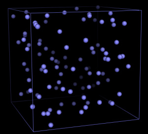
The first analysis step during or after a simulation is usually a visual inspection of the trajectory. For this, we will use VMD as a trajectory viewer. Other possibilities would be PyMol or gOpenmol.

vmd argon_start.pdb traj_comp.xtc

Select Graphics → Representations and then as Drawing Method: VDW. As standard, the view of the system is shown as perspective. To change this click Display → Orthographic. To display the box click Extensions → Tk Console and type in:

pbc box

(Alternatively, type pbc box into vmd > prompt that appeared in your Linux terminal). You can display the trajectory as a movie by pressing the arrow symbol at the bottom of the main VMD window. To change the speed of the movie you find a controller next to the arrow symbol.

We have simulated Argon at 100K, which is above the boiling point, so we have simulated argon gas. In the next step, we are slowly going to cool down the system (simulated annealing), to see if we can simulate the condensation to liquid Argon. Before we continue, change the directory to the parent directory (your home) with cd .. and create another directory for this new simulation: mkdir argon_cool. Now go to the newly created directory with cd argon_cool. You can now download anneal.mdp.

Do you remember what other files we need to start the simulation? The structure file and the topology file indeed. We will use the same starting structure and the same topology, so you can copy those files from argon_100K to the current directory with: (don’t forget the dot).

cp ../argon_100K/{argon_start.pdb,argon.top} .

The cp command takes here first the files you want to copy and second the destination, the dot means “current directory”. We can now create our unified .tpr input file:

gmx grompp -f anneal.mdp -c argon_start.pdb -p argon.top -maxwarn 1

Now start the annealing simulation:

gmx mdrun -v -c argon_anneal.gro

(note that we do not need to specify -s topol.tpr - as mdrun needs a tpr file to run, it will automatically search for the default filename: topol.tpr). Check the result with:

vmd argon_start.pdb traj_comp.xtc

Do you see the formation of liquid argon? To learn about an alternative visualization tool, let’s view the trajectory with PyMol. To do so, we first need to convert the trajectory to PDB format:

gmx trjconv -s -f traj_comp.xtc -o traj.pdb

and select 0. Then view the trajectory with PyMol:

pymol traj.pdb

On the white command prompt in PyMol, type:

show spheres
show cell

Press the play button on the bottom-right of the main PyMol window. Now analyze the energies and temperature from the simulation:

gmx energy -o temperature.xvg

and select the number for the temperature (and an extra Return stop the selection). Watch the result with:

xmgrace temperature.xvg

It can be seen that the actual temperature during the simulation indeed monotonously decreases as the simulation progresses. Now analyze the potential energy:

gmx energy -o potential.xvg

and select 4 (and 0 to stop the selection). Watch the result with:

xmgrace potential.xvg

Question: Why is there a drop in the potential energy?

💡 Recall that the Van-der-Waals potential is negative at small distances (close to the equilibrium distance), corresponding to a binding site. So how would the sum of all Van-der-Waals potentials change during condensation and boiling?

xmgrace temperature.xvg potential.xvg -legend load

Now repeat the annealing simulation, but extend the length of the simulation by a factor of five. Again, first, go to the parent directory (this should be your home directory) with cd .., create another directory with mkdir argon_cool_slow and change the directory cd argon_cool_slow. Copy the structure, topology and mdp files from the last simulation to the current directory with:

cp ../argon_cool/{argon_start.pdb,argon.top,anneal.mdp} .

Modify the following lines in the .mdp file to increase the simulation time:

nsteps = 2500000
annealing_time = 0 5000

Save anneal.mdp. And run the simulation:

gmx grompp -f anneal.mdp -c argon_start.pdb -p argon.top -maxwarn 1
gmx mdrun -v -c argon_anneal.gro

Analyze like above with gmx energy and xmgrace, using other output file names (e.g., temperature_slow.xvg, potential_slow.xvg).

Question: What is the boiling temperature this time? Why is the apparent boiling point higher than in the previous simulation?

egrep -v '#|@' temperature.xvg > temperature.dat
egrep -v '#|@' potential.xvg > potential.dat
paste temperature.dat potential.dat | awk '{print $2, $4}' > pot-vs-temp.dat
xmgrace pot-vs-temp.dat

Now, let us simulate the boiling instead of condensation of argon. For this, go to your home directory, create a new directory (mkdir argon_heat_long), go to this latest directory, download heatup.mdp and this time copy the topology and the output structure from the last long cool-down simulation:

cp ../argon_cool_slow/{argon_anneal.gro,argon.top} .

Start the simulation:

gmx grompp -f heatup.mdp -c argon_anneal.gro -p argon.top -maxwarn 1
gmx mdrun -v -c argon_heatup.gro

Analyze the results as above with gmx energy and xmgrace.

D. Freezing and melting of Argon

In the annealing simulations, we have not only observed the condensation to the liquid phase, but at lower temperatures also the freezing towards the solid phase. To concentrate on this phase transition more explicitly, we are now going to simulate the condensed phase. A simulation box has already been prepared. Download liquid.gro, and 94k.mdp to a newly created directory (go to your home, create the following directory: argon_liquid and download here or copy from another download directory location). Update the topology (argon.top) by changing the number of atoms (last line) from 100 to 216. Start the simulation of liquid argon with:

gmx grompp -f 94k.mdp -c liquid.gro -p argon.top -maxwarn 1
gmx mdrun -v -c liquid.pdb

To analyze the dynamic behavior of liquid argon, we’ll calculate the diffusion constant from the simulation. The Einstein formula can be used, which relates the mean atomic displacement to the diffusion constant. For this, we’ll use the program msd:

gmx msd -s -f traj_comp.xtc -trestart 50 -b 100

The option -trestart 50 means that time windows of 50 ps are used for the analysis (to enhance the statistics), and -b 100 means that the first 100 ps are excluded from the analysis. Select 0 or 1 when asked for a group.

Question: What is the calculated diffusion constant? How does it compare to the experimental value of $2.43*10^{-5} cm^2/s$?

Take a look at the mean-square displacement as a function of time:

xmgrace msd.xvg

One way to analyze the structural properties of a liquid is the so-called radial distribution function, which shows the probability of finding an atom center at a certain distance around an atom.

gmx rdf -s -f traj_comp.xtc -b 100 -o rdf_liquid.xvg

Select 0, 0 followed by Ctrl-D to start the calculation.

(Note that if the last command didn’t work (didn’t produce output for more than 30 seconds), please download a working version of gmx rdf (called g_rdf) from here, and make it executable with:

chmod +x g_rdf

and repeat the command from above with g_rdf).

xmgrace rdf_liquid.xvg

Now let us slowly cool the system. Setup a new simulation directory in your home directory as we used to do since the beginning of this practical and download anneal2.mdp and start the simulation:

gmx grompp -f anneal2.mdp -c liquid.gro -p argon.top -maxwarn 1
gmx mdrun -v -c anneal2.pdb

Check the animation (with PyMol or VMD) and the potential energy.

Question: When does the freezing begin? When would you have expected the freezing to start?

💡 Check the phase diagram

Compute the radial distribution function for the solid state, by taking into account only the second half of the simulation:

gmx rdf -s -f traj_comp.xtc -b 500 -o rdf_solid.xvg

and view the result together with the RDF of the liquid state:

xmgrace rdf_solid.xvg ../argon_liquid/rdf_liquid.xvg -legend load

E. Optional

Using a simulation strategy similar to the above, try to answer the following questions:

• Pressure dependence

  From the phase diagram, it is clear that in addition to the temperature, the phase behavior of argon is also strongly dependent on the pressure. Is this properly accounted for in the simulations? Try to see how the boiling point and the melting point at 1000 bar differ from the phase transitions at an ambient pressure of 1 bar. Is the observation consistent with the experiment? (💡: look for the word “pressure” in the GROMACS input .mdp file. If necessary, also check here.

• Sublimation

  At low pressures, there is no liquid state of argon, instead, there is a direct transition from the solid state to the gas phase, a process called sublimation. Is this also observed in the simulation?

• Simulation of Neon

  How are the results different for the much smaller neon? (💡: use this set of simulation parameters: neon.top).

• Collision of two droplets

  Investigate if you can use the kinetic energy of a moving droplet to induce a phase transition. To investigate this, shoot two droplets towards each other with different opposite velocities. With which velocities do you get a larger, merged droplet and from which velocities do you get a transition into the gas phase? 💡: use this structure file containing two droplets to start from. You’ll also need this index file, this topology file, and this parameter file.

Further References

• M. Karplus and A. McCammon. Molecular Dynamics simulations of biomolecules, Nature structural biology 9: 646-652 (2002).[link]
• D.C. Rapaport The Art of Molecular Dynamics Simulations - 2nd edn, Cambridge University Press (2004).
• H. Scheraga, M. Khalili and A. Liwo Protein-Folding Dynamics: Overview of Molecular Simulation Techniques, Annual Review of Physical Chemistry 58: 57-83 (2007).[link]