Topological-transitions workshop · Part 2 of 2
This guide follows the pore-formation tutorial. You can return to Part 1 at any time.
Introduction
Recall that the chain coordinate ξch quantifies the degree of connectivity between two membranes. During pore formation, a polar connection is formed between the two water compartments separated by a membranes. During stalk formation an apolar connection connection is formed between the hydrophobic cores of two membranes - hence, we can again use ξch to drive stalk formation in an MD simulation and to compute the respective PMF.
Run the stalk-formation showcase
This workflow uses the chain coordinate to connect two facing membrane leaflets and form a lipid stalk. It uses Martini 2 double-membrane systems.
Run these commands from the expanded participant workshop directory. The pore
and stalk workflows are independent; stalk scripts are numbered 20 and above.
1. Choose a system and create a private run
| System ID | Membrane |
|---|---|
dipc-stalk | DIPC |
dopc-stalk | DOPC |
dope-stalk | DOPE |
popc-stalk | POPC |
plasmamembraneinner-stalk | plasma-membrane inner mixture |
plasmamembraneouter-stalk | plasma-membrane outer mixture |
Set SYSTEM to one exact ID. RUN must be a new private directory:
SYSTEM=popc-stalk
RUN="$PWD/runs/$SYSTEM"

./scripts/20_stalk_create_run.sh "$SYSTEM" "$RUN"
The packaged system inputs are copied into the private run. Shared workshop inputs are never modified.
2. Choose the number of slices
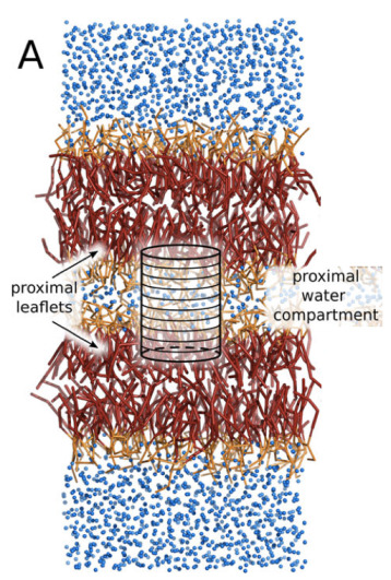
The chain coordinate divides a cylinder between the two membranes into N
slices and measures their hydrophobic lipid-tail occupancy. Here
you will determine a suitable N for your selected system. A good choice for
N corresponds to a cylinder that spans the entire polar region between
the two membranes and, in addition, slighly penetrates into the two hydrophobic cores.
Submit the intact-system scan:
./scripts/21_stalk_scan_slices.sh "$RUN" --submit
This starts 31 short CPU tasks. Every task analyses carries out a so-called rerun
from a given trajectory of two planar membranes, trying values for N from N=20
through N=50; it does not run 31 new molecular-dynamics simulations. Mathematically,
it projects the simulation frames on the coordinate ξch,N using different
values of N.
Check progress:
./scripts/21_stalk_scan_slices.sh "$RUN" --status
Wait until the summary reports:
Completed: 31 / 31
Running:   0
Pending:   0
Other:     0
Then collect the results:
./scripts/21_stalk_scan_slices.sh "$RUN" --collect
A FAIL row means that particular slice count N is too small, that the cylinder
does not span the space between the two membranes. As you see, when using different values for
N, ξch yields different values for the state with the two planar membranes.
Now, choose N such that ξch is close to 0.2, meaning that ~20% of the
slices are filled by apolar atoms in the state with two planar membranes (the “unconnected”
state). This places the
unconnected state near the lower part of the coordinate while leaving room for
ξch to increase as the stalk forms.
For example, to choose N=36:
./scripts/21_stalk_scan_slices.sh "$RUN" --choose 36
The command verifies that the selected value passed the scan before updating
$RUN/input/coordinate.env. It records your choice; it does not choose N
automatically.
3. Understand the opening rate
Again, we use a time-dependent harmonic potential to drive the system towards a stalk $$ V(\mathbf{r}) = \frac{k}{2}(\xi_\mathrm{ch}(\mathbf{r}) - \xi_\mathrm{ch,ref}(t))^2, $$ where we gradually move the target value (or reference value) $\xi_\mathrm{ch,ref}(t)$ from 0.1 to 1.0. The opening simulation lasts 50 ns.
opening rate = (final target - initial target) / duration
             = (1.0 - 0.1) / 50000 ps
             = 1.8e-05 per ps
This opening is deliberately fast so that the exercise remains feasible with limited computational resources. A slower change in the target $$ would give the membrane more time to relax and could provide better equilibrated starting structures.
The measured ξch follows the moving target but does not have to equal it at every instant. The opening trajectory supplies starting structures for the umbrella windows; it is not used directly to calculate the PMF. Later, each umbrella window keeps its target ξch fixed.
The workshop uses the fixed opening rate of 1.8e-05 per ps. Before preparing the
simulation, check that your run configuration is complete:
./scripts/22_stalk_validate_configuration.sh "$RUN"
This command does not start a simulation. It runs sanity checks before we submit.
Do not continue until the configuration check succeeds.
4. Prepare and submit the opening
First, compile the coordinates, topology, selected slice count, and simulation
settings into a GROMACS run-input file (opening.tpr):
./scripts/23_stalk_prepare_opening.sh "$RUN"
This command checks and prepares the simulation; it does not run molecular dynamics. It prints the pulling groups, thermostat groups, moving target, output path, and location of the complete GROMACS preprocessing log.
Submit the prepared 50 ns simulation:
./scripts/24_stalk_submit_opening.sh "$RUN"
Check its status (feel free to run this command as often as needed):
./scripts/25_stalk_check_opening.sh "$RUN"
The progress summary distinguishes the prescribed target from the reaction
coordinate measured in the simulation. For example, a value of -0.04 for
measured minus target means that the measured ξch is 0.04 below
the current target.
Some lag is expected because the workshop opening moves the target quickly,
while lipids and water need time to rearrange. During the run, check that the
measured ξch generally increases by looking into the pullx.xvg file.
A coordinate that stops increasing
or falls far behind the target may leave some umbrella windows without
suitable starting structures.
The command also reports the simulated time, completion percentage,
performance when available, and the current Slurm state. Wait until it reports
Own stalk opening: complete.
After the opening finishes, select it as the source of umbrella structures:
./scripts/25_stalk_check_opening.sh "$RUN" --select-own
The stalk workflow currently has no packaged fallback opening. An incomplete or failed opening must be inspected before continuing.
5. Watch the stalk form in VMD
The opening trajectory provides a direct view of the transition from two separated membranes to a lipid connection.
On Rosi
From the expanded workshop directory, run:
./scripts/31_stalk_prepare_vmd.sh "$RUN"
The command creates a PDB containing explicit Martini bonds and a processed XTC
trajectory. It also prints SYSTEM=... and REMOTE_OPENING=... lines for the
next step.
On your computer
Open a new terminal on your own computer, not inside the Rosi SSH session.
Copy and run the SYSTEM=... and REMOTE_OPENING=... lines printed on Rosi.
Set ROSI_LOGIN to the same hostname or SSH alias that you normally use to
connect to Rosi:
ROSI_LOGIN=rosi
LOCAL_OPENING="$HOME/workshop-visualization/$SYSTEM/opening"

mkdir -p "$LOCAL_OPENING"

scp \
    "${ROSI_LOGIN}:${REMOTE_OPENING}/structure-conect.pdb" \
    "${ROSI_LOGIN}:${REMOTE_OPENING}/trajectory-whole.xtc" \
    "$LOCAL_OPENING/"
Verify that both files were copied:
ls -lh "$LOCAL_OPENING"
Start VMD on your computer:
vmd \
    "$LOCAL_OPENING/structure-conect.pdb" \
    "$LOCAL_OPENING/trajectory-whole.xtc"
Load the PDB first because it supplies the Martini bond connectivity. The XTC then adds the trajectory frames. Play the trajectory and identify the two facing membrane leaflets, the intervening water, and the lipid connection that develops during the opening.
6. Generate the umbrella grid
The default table describes 19 windows from ξ=0.10 through ξ=1.00, with spacing 0.05 and force constant 3000 kJ mol⁻¹.
./scripts/26_stalk_generate_window_grid.sh "$RUN"
cat "$RUN/state/window-grid.tsv"
The window count is derived from input/window-regions.tsv; the scripts do not
assume there are always 19 windows.
7. Submit and monitor the umbrella windows
./scripts/27_stalk_submit_windows.sh "$RUN"
Each array task selects a unique saved opening frame, renders its target restraint, prepares a TPR, and runs one 20 ns umbrella simulation.
No minimization is inserted between extraction and umbrella sampling. The first 20% of each window is excluded from WHAM.
Monitor completion:
./scripts/28_stalk_status.sh "$RUN"
Do not start WHAM until every expected window has finished, every window has a
non-empty pullf.xvg, and no fatal log is reported.
Analyse the stalk-formation PMF
Run the analysis only after every umbrella window has completed.
1. Check window completion
./scripts/28_stalk_status.sh "$RUN"
The expected, finished, and pull-force counts must agree. No fatal log should be reported. The expected count is read from the generated grid and is not permanently fixed at 19.
2. Run WHAM
./scripts/29_stalk_analyze.sh "$RUN"
The script reads the umbrella duration from input/umbrella.mdp. With the
provided protocol, every window lasts 20 ns.
| Interval | Use |
|---|---|
| 0–4 ns | discarded |
| 4–20 ns | retained for the main PMF |
| 4–12 ns | first convergence block |
| 12–20 ns | second convergence block |
WHAM therefore uses 16 ns of force data from each completed window.
The two retained 8 ns blocks provide a simple convergence check: their
disagreement is summarized in $RUN/analysis/analysis-summary.txt, and the
underlying profiles are saved as pmf-first-half.xvg and
pmf-second-half.xvg.
3. Inspect the report
Open:
RUN/analysis/report.html
The report contains the stalk-formation PMF, bootstrap uncertainty, adjacent-window overlap, and the analysis settings.
Important output files are:
| File | Meaning |
|---|---|
pmf-bootstrap-reference-zero.tsv | PMF and bootstrap standard deviation |
histograms.xvg | sampled coordinate distributions |
overlap-summary.tsv | overlap between adjacent windows |
pmf-first-half.xvg | PMF from the first retained 8 ns |
pmf-second-half.xvg | PMF from the second retained 8 ns |
analysis-summary.txt | machine-readable analysis record |
report.html | offline participant report |
Understand the PMF
The horizontal axis follows stalk formation: low ξch describes separated membrane leaflets, while values approaching one describe increasing connectivity between them.
The PMF reports relative free energy along this coordinate. Lower regions are more favourable within the sampled pathway; an increase means that progressing along the coordinate requires free energy. Only differences are meaningful, so the vertical origin is shifted using the minimum between ξ=0.10 and ξ=0.30.
This zero is a plotting convention. It does not prove that the minimum is an absolute thermodynamic reference or a fully converged equilibrium state.
Check overlap and convergence
Each restrained window samples a distribution of ξch values rather than one exact value. Neighbouring umbrella histograms must overlap so that WHAM can connect them into one PMF.
The adjacent-window chart counts histogram bins occupied by both members of each neighbouring pair. A zero-height bar is a gap and the PMF must not be interpreted. A nonzero bar is necessary, but does not by itself prove adequate sampling or convergence.
The analysis also compares PMFs calculated from the first and second retained 8 ns blocks. Similar profiles support convergence over this limited interval; large local differences identify regions that require longer sampling.
In addition, we estimate the uncertainty by bootstrapping complete histograms. Technically, this is done by assigning random weights to the histograms, followed by a WHAM run giving a new “synthetic” PMF, and repeated 50 times. The standard deviation among the 50 synthetic PMFs is a remarkably robust error estimate for the PMF because it only assumes that complete histograms are statistically independent.
Interpretation and limitations
The starting systems and force-field setups are derived from the published stalk-formation study by Poojari et al., Nature Communications 12, 6594 (2021). The shortened protocol used here is designed for teaching; it is neither a reproduction nor an independent publication-quality validation of that study.
In particular:
- each system uses a single opening trajectory;
- each umbrella window lasts only 20 ns;
- the first 4 ns of each window is discarded;
- no independent replicas are included;
- critically, no reverse stalk-closure pathway is sampled, so hysteresis is not assessed.
Wrapping up, you learned how to carry out free energy calculations of the first step of membrane fusion, i.e., the formation of the fusion stalk. Congratulations to successfully finishing the tutorial!
References
Poojari, Scherer, Hub, Free energies of membrane stalk formation from a lipidomics perspective, Nat. Commun., 12, 2041-1723 (2021), DOI:10.1038/s41467-021-26924-2
Scherer, Poojari, Hub, Transmembrane domains of fusion proteins promote stalk formation by inducing membrane disorder, Biophysical Journal 125, 1276-1285 (2026), DOI:10.1016/j.bpj.2026.01.032
Hub, J. S. and Awasthi, N. (2017). “Probing a Continuous Polar Defect: A Reaction Coordinate for Pore Formation in Lipid Membranes.” Journal of Chemical Theory and Computation. DOI: 10.1021/acs.jctc.7b00106
Force-field reference
The stalk systems use the Martini 2.2 force field:
Marrink, S. J., Risselada, H. J., Yefimov, S., Tieleman, D. P., and de Vries, A. H. (2007). “The MARTINI Force Field: Coarse Grained Model for Biomolecular Simulations.” Journal of Physical Chemistry B 111, 7812–7824. DOI: 10.1021/jp071097f
Workshop navigation
Return to the pore-formation guide to revisit Part 1.