Topological-transitions workshop · Part 1 of 2
Start here with pore formation. After completing this guide, continue with stalk formation.
Start the workshop on Rosi
Connect to Rosi in an SSH terminal and initialize your private workshop copy:
. /home/tut04/pore-workshop/start
The launcher verifies release 0.9.0, installs it as
~/pore-workshop-0.9.0, enters that directory, and runs the cluster preflight.
Leave this terminal open for the simulation commands below.
Introduction and Background: transmembrane pore formation
A membrane pore is a topological transition: an intact bilayer becomes connected by a water-filled polar defect. The chain coordinate ξch turns that connectivity into a continuous value that can be restrained and used to calculate a potential of mean force (PMF).
The formation of membrane pores plays key roles in numerous processes of biological or medical relevance: Pores are formed during apoptosis, by antimicrobial peptides, or during membrane fusion (which in turn is involved in signaling, viral infection, and fertilization). During electroporation, pores are formed with an external electric pulse with the aim delivering cargos into cells. In MD simulations, pores do not form spontaneously because pore formation is typically associated with a high free energy cost. Therefore, to observe pores formation in MD simulations and to study the roles of lipids, membrane-active pepties, or electric fieds on pore formation, pore formation must be simulated by pulling along reaction coordinate (or collective variable): the chain coordinate.
A fromation of a transmembrane pore is a topological transition: an intact bilayer becomes protruded by a water-filled continuous polar defect. The chain coordinate ξch turns the degree of connectivity of the transmembrane defect into a continuous value that can be restrained and used to calculate the potential of mean force (PMF) of pore formation.
Warning: In this tutorial, we use the MARTINI coarse-grained force field to simulate pore fomation owing to the low computational costs. For a scientific study of pore formation, we strongly discourage the use of MARTINI, see below.Warmup: watch an equilibrium membrane
Before opening a pore, look at a normal Martini 3 bilayer moving at equilibrium. VMD runs on your own computer; the simulations remain on the cluster.
- Download and install the appropriate VMD build from the official VMD alpha download.
- Add the directory containing the
vmdexecutable to your local shell’sPATH. For example, replace the example directory below with the actual installation directory:
export PATH="/opt/vmd/bin:$PATH"
command -v vmd
To keep this setting, add the same export PATH=... line to ~/.bashrc for
Bash or ~/.zshrc for Zsh, then open a new terminal. The installation directory
depends on your operating system and chosen VMD package.
Open another terminal on your own computer and copy the prepared example from
Rosi. Set ROSI_LOGIN to the hostname or SSH alias you normally use for Rosi:
ROSI_LOGIN=rosi
LOCAL_EXAMPLE="$HOME/workshop-visualization/equilibrium-membrane"

mkdir -p "$LOCAL_EXAMPLE"
scp \
    "${ROSI_LOGIN}:pore-workshop-0.9.0/reference/equilibrium-vmd/equilibrium-conect.pdb" \
    "${ROSI_LOGIN}:pore-workshop-0.9.0/reference/equilibrium-vmd/equilibrium-whole.xtc" \
    "$LOCAL_EXAMPLE/"

vmd \
    "$LOCAL_EXAMPLE/equilibrium-conect.pdb" \
    "$LOCAL_EXAMPLE/equilibrium-whole.xtc"
If you already mount your Rosi home directory with SSHFS or an SFTP filesystem
client, you may open the same two files directly from
pore-workshop-0.9.0/reference/equilibrium-vmd/. Run all simulation commands in
the Rosi SSH terminal, not on your local computer.
VMD now shows and example of a previously carried out equilibriums simulation of a membrane of POPC, without any pore-opening restraint. Play or scrub the trajectory, rotate the bilayer, and identify water, headgroups, and the hydrophobic core.
The example includes equilibrium.gro, a one-frame GROMACS structure, and
equilibrium-whole.xtc, the trajectory. VMD loads
equilibrium-conect.pdb first because a GRO or XTC does not carry the Martini
bond topology.
Advanced: why the VMD structure is a PDB
VMD may guess missing or incorrect bonds for coarse-grained molecules. The
provided PDB was generated from a compiled topology (.tpr) with
gmx trjconv -conect, which writes explicit CONECT records. The trajectory
was made whole with -pbc whole and then centred in a separate -pbc mol -center pass. The generated ENDMDL record was removed so VMD applies the PDB
connectivity to every XTC frame.
For another trajectory, the portable helper performs the same preparation:
./scripts/14_prepare_vmd.sh topol.tpr traj.xtc index.ndx visualization
vmd visualization/structure-conect.pdb visualization/trajectory-whole.xtc
Always load the CONECT-enabled PDB first and the processed XTC second.
From polar connectivity to pore size
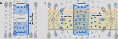
The chain coordinate ξch measures the degree of connectivity of the transmembrane defect. To quantify “connectivity”, it uses the fraction of polar-occupied slices in a membrane-spanning cylinder (see left image). In case you also want to simulate pore expansion, an extension of the chain coordinate may be used to switch from pore nucleation (left image) to pore expansion (measured as as the pore radius), together implemented as a joint coordinate ξp for pore nucleation and expansion. Adapted from Hub, JCTC 2021.
In the published atomistic definition, water oxygen and lipid phosphate oxygen atoms contribute when they lie inside the cylinder. An intact membrane leaves central slices empty; water entry occupies more slices; ξch approaches unity when the defect spans the entire membrane. The chain coordinate then saturates and cannot describe further pore expansion. The joint coordinate ξp solves that problem by switching smoothly to the expansion term.
Explore the full published pathway
Use the slider to follow atomistic structures from an intact membrane through pore nucleation and expansion. The values at the bar are ξp; in this workshop, however, we only use the chain coordinate ξch to focus on the pore nucleation phase.
What you will do
The workshop has two successive applications of the chain coordinate.
First, you will study pore formation in a Martini 3 membrane. You will choose the cylinder resolution and opening rate, generate 27 short umbrella windows, and reconstruct a pore-formation PMF.
After completing that workflow, you will apply the same ideas to stalk formation between two facing Martini 2 membranes. You will calibrate the coordinate for a double membrane, follow a 50 ns stalk-opening trajectory, generate 19 umbrella windows, and reconstruct a stalk-formation PMF.
The workflows use separate run directories and scripts, so their simulation files remain independent. Conceptually, the stalk exercise builds on what you learned during the pore exercise.
Everything else uses tested defaults. Optional explanations are available in expandable Advanced panels.
Run the showcase
Keep this page open beside a terminal. Commands beginning with ./scripts/
must be run from the copied workshop folder.
1. Choose a membrane and create your run
| Membrane | Enter exactly as SYSTEM | A useful comparison |
|---|---|---|
| DIPC | dipc-small | two polyunsaturated tails |
| DLPC | dlpc-small | short saturated tails |
| PAPC | papc-small | one highly unsaturated tail |
| POPC | popc-small | common phosphatidylcholine reference |
| POPE | pope-small | smaller PE headgroup |
| POPG | popg-small | negatively charged headgroup |
SYSTEM is the exact membrane ID. RUN is the new private directory that will
hold your calculation. For example:
export SYSTEM=popc-small
export RUN="$(realpath -m "$PWD/../${USER}-${SYSTEM}")"
./scripts/01_create_run.sh "$SYSTEM" "$RUN"
./scripts/02_inspect_system.sh "$RUN"
Replace only popc-small. Your run is independent and is never combined with
another participant’s files.
GROMACS file types
| File | Role |
|---|---|
.gro | one molecular structure and the simulation box |
.top / .itp | molecular composition and force-field definitions (topology) |
.ndx | definitinos of groups of atoms or beads (index groups) |
.mdp | simulation and restraint settings |
.tpr | compiled run input produced by grompp |
.xtc | compressed trajectory produced by mdrun |
.xvg | coordinate or force data used for analysis |
structure + topology + groups + settings  →  grompp  →  .tpr
                                                       ↓ mdrun
                                                .xtc + .xvg
Advanced: shell variables and inspecting every input
The leading $ asks Bash to substitute a variable’s value. If user alice
chooses POPC, $SYSTEM becomes popc-small and $RUN might become
/home/alice/alice-popc-small. Braces in ${USER} mark where a variable name
ends; quotation marks keep a path together.
printf 'SYSTEM=%s\nRUN=%s\n' "$SYSTEM" "$RUN"
ls -lh "$RUN/base"
tail -1 "$RUN/base/equilibrated.gro"
less "$RUN/base/topol.top"
less "$RUN/base/index.ndx"
The base is an equilibrated 162-lipid membrane with its normal along z. The
index must contain tails, Solvent, Non-Solvent, and Phosphates. POPG
also contains counterions. Press q to leave less.
2. Choose the number of slices (or length of the cylinder)
The membrane-spanning cylinder is divided into N slices with thickness of 2Å (1Å for all-atom simulations). Hence, the definition of ξch requires choosing N. Choose N (and thereby the length) such that, for a planar intact membrane (with no pore), ξch takes a value of ~0.2 meaning 20% of the cylinder slices are occupied by polar atoms, namely the slices in the two head group regions. This ensures that the cylinder spans the entire membrane including some parts of the polar headgroup reagion. If the cylinder is too short such that no slice contains a polar atom, you get an error message. In practice, you run a series of so-called reruns from a given equilibrium simulation trajectory, compute ξch with various values of N form the frames. Then choose a good value. We did this for you in advance:
Inspect the results from these reruns, which we did in advance for you:
./scripts/03_scan_slices.sh "$RUN" --reference
column -t -s $'\t' "$RUN/calibration/scan-status.tsv" | less
Look for three things:
- reject values marked
FAIL- cylinder is too short,Ntoo small; - observe how the computed ξch changes with the choice of
N; - choose a passing
Nwith an mean close to 0.2–0.25, making sure that the cylinder spans the membrane.
Make a provisional choice and replace CHOOSE_FROM_SLICE_SCAN:
${EDITOR:-nano} "$RUN/input/coordinate.env"
./scripts/03_scan_slices.sh "$RUN" --check-choice
Try another plausible value if you want to compare. Your first choice does not have to match the tested one. Decide from the evidence before opening the solution, then reconcile your value before selecting a fallback opening.
Show the tested slice-count solution
The release selects the passing value whose intact mean is closest to 0.25:
./scripts/03_scan_slices.sh "$RUN" --solution
cat "$RUN/calibration/selected-slices.tsv"
| System | Good value for N | mean ξch |
|---|---|---|
| DIPC | 16 | 0.269 |
| DLPC | 15 | 0.226 |
| PAPC | 18 | 0.254 |
| POPC | 18 | 0.242 |
| POPE | 19 | 0.234 |
| POPG | 17 | 0.233 |
If your choice for N strongly differs, compare it with the calibration criterion
and use the tested value for the packaged fallback workflow.
Advanced: environment variablers for defining the reaction coordinate
The scan measures ξch on an intact trajectory for candidate slice
counts. A passing value with an intact mean near 0.2–0.25 stays well separated
from a connected defect at ξch≈1. The full scan can be reproduced with
--submit, then --collect after its Slurm array finishes.
coordinate.env setting | Meaning and default |
|---|---|
SLICE_COORD_N | number of slices; important! |
SLICE_COORD_D | slice thickness, 0.2 nm for MARTINI, 0.1 nm for all-atom |
SLICE_COORD_CYL_R | cylinder radius, typically ~1.0 nm |
| Advanced options: | |
SLICE_COORD_ZETA | fraction to which a slice is filled upon addition of the first atom, 0.75 |
SLICE_COORD_NST_OUTPUT | coordinate-output interval written to stdout |
SLICE_COORD_FREEZE_CYLINDER_X/Y | freeze lateral position of the cylinder at these x and y positions |
SLICE_COORD_FREEZE_CYLINDER_XIREF | freezes cylinder laterally only if reference positino of ξch is below this value |
SLICE_COORD_COUNTERFORCE | applies the balancing coordinate force |
SLICE_COORD_CYLINDER_FORCE | includes the radial cylinder-boundary force |
The MDP files defines the atom groups used to compute ξch: Here, we use
Solvent as group of polar atoms (contributing to ξch) and tails as
the membrane reference pull group. (For all-atom simulations a good choice for the polar atoms
is the water oxygens and lipid phosphate oxygens.) In this workshop with Martini 3, we use
coarse-grained water beads (plus counterions for POPG) as polar atoms; Phosphates is
supplied for inspection.
The lateral cylinder position is frozen at the box centre while ξch<0.7. After that, the cylinder may move in the membrane plane, which is important since also the defect may laterally travel in the membrane plane. This behavious is critital to avoid undesired hysteresis effects.
3. Choose the opening rate
The pore-opening pulling simulation applies an harmonic restraint along ξch to gradually force the simulation towards pore formation: $$ V(\mathbf{r}) = \frac{k}{2}(\xi_\mathrm{ch}(\mathbf{r}) - \xi_\mathrm{ch,ref}(t))^2, $$ where we gradually move $\xi_\mathrm{ch,ref}(t)$ from 0.1 to 1.0. Inspect the timestep and number of steps in the MDP file:
grep -E '^[[:space:]]*(dt|nsteps|pull-coord1-init)' \
    "$RUN/input/opening.mdp"
First calculate the duration dt × nsteps in ps. Then calculate:
pull rate = (desired final value − initial value) / duration in ps
Replace CHOOSE_OPENING_RATE_XI_PER_PS in the MDP file with your result and test it. An
incorrect value is safe here: the validator reports the endpoint and refuses to
prepare a simulation until it is close to 1.0.
${EDITOR:-nano} "$RUN/input/opening.mdp"
./scripts/04_validate_configuration.sh "$RUN"
Revise the rate if validation fails. Reveal the solution only after making a first calculation.
Show the opening-rate solution
dt = 0.015 ps and nsteps = 1,333,333 give approximately 20,000 ps.
(1.0 − 0.1) / 20,000 ps = 4.5 × 10⁻⁵ ps⁻¹
Enter 4.5e-05 as pull-coord1-rate, then rerun
04_validate_configuration.sh.
Once both choices validate, prepare and submit. Here the prepare and submit scripts essentially run the Gromacs commands gmx grompp and gmx mdrun, but help you with getting files into the right folders:
./scripts/05_prepare_opening.sh "$RUN"
./scripts/06_submit_opening.sh "$RUN"
./scripts/07_check_opening.sh "$RUN"
If the status says your opening is complete, select it:
./scripts/07_check_opening.sh "$RUN" --select-own
If it is still queued or running, select the validated opening simulation for the same membrane instead:
./scripts/07_check_opening.sh "$RUN" --use-fallback
Advanced: opening restraint, MDP flags, and saved data
The opening simuliation is a nonequilibrium simulation, using constant-velocity pulling fromξch=0.1 to ξch=1.0. This simulation is used below to obtain starting frames for umbrella sampling. For Gromacs users, here the MDP parameters used to the pulling simulation:
opening.mdp setting | Purpose |
|---|---|
integrator = md | molecular-dynamics integrator |
dt = 0.015 ps | integration step, 15 fs used here with Martini |
nsteps = 1333333 | fixed 20 ns duration |
pull-coord1-geometry = pore-slices | chain coordinate for polar-defect connectivity |
pull-group1-name = tails | pull group 1 |
pull-group2-name = Solvent | pull group 2 |
pull-coord1-groups = 1 2 | Use pull groups 1 and 2 as membrane reference and polar atoms, respectively |
pull-coord1-dim = N N Y | coordinate acts along the membrane normal |
pull-coord1-init = 0.1 | initial restraint centre |
pull-coord1-rate | participant-selected motion in ξch per ps |
pull-coord1-k = 3000 | force constant along ξch |
pull-nstxout/fout = 50 | coordinate and force output every 0.75 ps |
nstxout-compressed = 3300 | structure every 49.5 ps |
The validator checks duration, endpoint, groups, geometry, and output cadence. The frame selector uses measured ξch rather than assuming that the membrane follows the moving target without lag. It assigns one distinct opening frame to each umbrella target.
grep -E 'nsteps|pull-nstfout|pull-coord1-(geometry|init|rate|k)' \
    "$RUN/opening/opening.mdp"
GROMACS writes the coordinate to opening_pullx.xvg and the applied
force to opening_pullf.xvg. Take a look, e.g. with xmgrace:
xmgrace opening_pullx.xvg
and inspect the simulation with VMD. Do you see the pore?
4. Generate and submit the umbrella sampling simulations
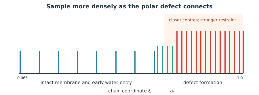
Umbrella windows restrain the system at neighboring ξch values. From each window, a histogram along ξch is collected. From all histograms the PMF is computed with the so-called weighted histogram analysis method (WHAM).
./scripts/08_generate_window_grid.sh "$RUN"
./scripts/10_submit_windows.sh "$RUN"
./scripts/11_status.sh "$RUN"
This creates 27 independent umbrella windows, each simulated for 2 ns. Slurm starts each one when a GPU is available.
Advanced: window spacing, force constants, generated files, and Slurm
To optimally sample the critical regions along the pore formation process, we do not use equidistant umbrella windows. Instead, at at small ξch, where the membrane is still intact, we use fewer windows (with smaller force constants); at larger ξch, where the defects is (nearly) connected, we use tighter windows (with larger force constants). The regional table expands to targets from ξch=0.065 to 1.0, so nobody edits 27 MDP files manually.
The umbrella master fixes dt = 0.015 ps, nsteps = 133333, zero pull rate,
pore-slices geometry, and force output every 0.75 ps. The representative
preview shows MDP settings for one early window, one intermediate, and one late umbrella window:
./scripts/09_prepare_representatives.sh "$RUN" --preview
column -t -s $'\t' "$RUN/input/window-regions.tsv"
less "$RUN/state/window-grid.tsv"
grep -H -E 'pull-coord1-(geometry|init|k)' \
    "$RUN"/state/representative-preview/*/umbrella.mdp
Each Slurm task extracts its assigned frame, carries out an energy minimization,
creates a run-input TPR file, and runs in its own directory. Production mdrun commands use a
bound srun step with explicit CPU and GPU binding so co-located tasks do not
compete for the same CPU cores.
See the result
Inspect a prepared result
If your simulations are still running, first inspect the prepared result for the same membrane:
cat "reference/results/$SYSTEM/analysis-summary.txt"
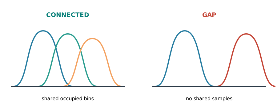
Open reference/results/$SYSTEM/report.html in a browser. A useful result has:
- all 27 windows completed;
- connected overlap between every neighboring pair;
- a PMF shown with uncertainty only over the sampled ξch range.
Analyze your result
Restore RUN, check completion, and build your report:
export RUN=/home/alice/alice-popc-small
./scripts/11_status.sh "$RUN"
./scripts/12_analyze.sh "$RUN"
Then open $RUN/analysis/report.html. You now have the complete workflow from
an equilibrated membrane to a diagnosed pore-nucleation PMF.
Congratulations, you carried out pulling simulations and umbrella sampling simulations along ξch to compute the PMF of pore formation with the MARTINI force field.
A few points to keep in mind:
- We used short simulations, hence the PMF is not fully converged.
- MARTINI works remarkably well for certain applictions, but may have severe shortcomings for other applications. Therefore, compare below with PMFs from all-atom simulations.
- We restricted the tutorial to pore nucleation but did not study pore expansion.
Critically compare PMF of pore formation obtaind with MARTINI with PMF from all-atom simulations
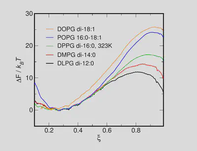
Figure S1 from Ting et al., PRL 2018: atomistic CHARMM36 PMFs for phosphatidylglycerol (PG) membranes.
This figure shows PMF of pore formation obtained with all-atom simulations. Check also the PDF of Ting et al. for PMFs with PC lipids. Note the local minima of the PMFs at ξch =1. What do these minima imply, for instance with respect to the life time of open pores?
Do you see such minimal in the PMFs obtained with MARTINI? Comare with your colleagues who possibly simulated other lipid types.
What can you say about the free energy cost of pore formation in MARTINI compared to all-atom CHARMM36 simulations? Note that $kT \approx 2.5 \mathrm{kJ/mol}$. Note that the probability of pore formation follows:
$$ P_\mathrm{pore} \propto \exp(-\Delta G/k_B T), $$
where $\Delta G$ is the free energy of pore formation. By which factor is the probability of pore formation underestimated by Martini?
Advanced: WHAM, edge support, uncertainty, and convergence
The analysis uses 400–2000 ps, discarding the first 20% for equilibration. WHAM combines the umbrella histograms after checking that adjacent windows overlap. It performs 50 rounds of bootstrapping for computing errors and compares the first and second halves of the retained interval.
An empty endpoint bin can look like an unphysical PMF drop. The script therefore finds the sampled range first, requires at least 20 aggregate force records at each reported edge, and withholds the report if any zero-count bin remains. The supported endpoint can be slightly below ξch=1 and differs by membrane.
Inspect the diagnostics directly with:
cat "$RUN/analysis/analysis-summary.txt"
column -t "$RUN/analysis/overlap-summary.tsv" | less
grep -RE 'Fatal error|Segmentation fault|CUDA error' "$RUN"
find "$RUN/windows" -name 'pullf.xvg' -size +0c | wc -l
A smooth PMF is does not imply convergence. Things to critically check include: Do histograms overlap? Do PMFs obtained from different time blocks agree? Is the uncertainty from bootstrapping acceptable? The 2 ns simulations carried out here are certaintly quite short, and longer simulations are needed for full convergence. For all-atom simulatinos we typically carry out 150 ns per umbrella window.
Next: form a stalk
Now that you have used the chain coordinate to describe pore formation, apply the same principles to a different topological transition: stalk formation between two facing membranes. The simulations use separate files, but the coordinate-calibration, umbrella-sampling, and PMF concepts carry over.
Continue to Part 2: stalk formation →
Optional: continue with pore expansion
The workshop stops at a connected polar defect. The extended GROMACS Chain Coordinate example continues with the joint reaction coordinate ξp for pore nucleation and expansion, including its smooth switch from ξch to pore-radius expansion, and provides a more extensive tutorial.
Optional advanced reference
This page is optional lookup material.
Essential terms
| Term | Meaning here |
|---|---|
| ξch | chain coordinate: fraction of polar-occupied cylinder slices |
| ξp | joint coordinate that switches from ξch to pore-radius expansion |
| polar defect | water and headgroups penetrating the hydrophobic core |
| opening | moving-restraint path used to create starting structures |
| umbrella window | equilibrium simulation restrained near one coordinate value |
| PMF | potential of mean force along a reaction coordinate |
| overlap | neighboring windows sampling common coordinate values |
| WHAM | method that combines the biased window histograms |
Advanced: complete command sheet
export SYSTEM=popc-small                 # replace with one listed system ID
export RUN="$(realpath -m "$PWD/../${USER}-${SYSTEM}")"
./scripts/00_preflight.sh
./scripts/01_create_run.sh "$SYSTEM" "$RUN"
./scripts/02_inspect_system.sh "$RUN"
./scripts/03_scan_slices.sh "$RUN" --reference
${EDITOR:-nano} "$RUN/input/coordinate.env"   # enter your provisional N
./scripts/03_scan_slices.sh "$RUN" --check-choice
./scripts/03_scan_slices.sh "$RUN" --solution # reveal only after choosing
${EDITOR:-nano} "$RUN/input/opening.mdp"      # calculate and test the rate
./scripts/04_validate_configuration.sh "$RUN"
./scripts/05_prepare_opening.sh "$RUN"
./scripts/06_submit_opening.sh "$RUN"
./scripts/07_check_opening.sh "$RUN"
# Select exactly one opening source:
./scripts/07_check_opening.sh "$RUN" --select-own
# or: ./scripts/07_check_opening.sh "$RUN" --use-fallback
./scripts/08_generate_window_grid.sh "$RUN"
./scripts/09_prepare_representatives.sh "$RUN" --preview
./scripts/10_submit_windows.sh "$RUN"
./scripts/11_status.sh "$RUN"
./scripts/12_analyze.sh "$RUN"
Stop before interpretation if the patched GROMACS executable is wrong, an
index group is missing, grompp warns, a placeholder remains, a window fails,
two starting structures are identical, or adjacent histograms have a gap.
Sources and further reading
Reaction coordinate
Hub, J. S. and Awasthi, N. (2017). “Probing a Continuous Polar Defect: A Reaction Coordinate for Pore Formation in Lipid Membranes.” Journal of Chemical Theory and Computation. DOI: 10.1021/acs.jctc.7b00106
Hub, J. S. (2021). “Joint Reaction Coordinate for Computing the Free-Energy Landscape of Pore Nucleation and Pore Expansion in Lipid Membranes.” Journal of Chemical Theory and Computation. DOI: 10.1021/acs.jctc.0c01134 · group-hosted PDF
Hub group. “Example system illustrating how to use the joint reaction coordinate for pore formation and expansion.” GROMACS Chain Coordinate tutorial
Applications and interpretation
Ting, C. L., Awasthi, N., Müller, M., and Hub, J. S. (2018). “Metastable Prepores in Tension-Free Lipid Bilayers.” Physical Review Letters 120, 128103. DOI: 10.1103/PhysRevLett.120.128103 · Supporting information
Starke, S., Allolio, C., and Hub, J. S. (2025). “How pore formation in complex biological membranes is governed by lipid composition, mechanics, and lateral sorting.” PNAS Nexus. DOI: 10.1093/pnasnexus/pgaf033
Foundations, convergence, and finite size effects
Awasthi, N. and Hub, J. S. (2016). “Simulations of Pore Formation in Lipid Membranes: Reaction Coordinates, Convergence, Hysteresis, and Finite-Size Effects.” Journal of Chemical Theory and Computation. DOI: 10.1021/acs.jctc.6b00369
The published coordinate and pore-state images are adapted from Hub, JCTC
2021. The atomistic PMF comparison is Figure S1 from the supporting information
of Ting et al., PRL 2018. Software versions and system provenance are recorded
in PROVENANCE.md.
MD simulations with Gromacs, visualization
University of Illinois. VMD alpha downloads and VMD command-line options. VMD accepts a PDB structure on its command line and can append a trajectory to that molecule.
GROMACS 2021 documentation for
gmx trjconv
and
gmx editconf.
The -conect option writes PDB bond records for non-standard molecules such as
coarse-grained lipids; -pbc whole makes broken bonded molecules whole.
SSHFS project. SSHFS usage and installation.
SSHFS exposes a remote SFTP directory as a local filesystem using
sshfs user@host:directory mountpoint.
Continue to stalk formation
You have completed Part 1. Continue with the second chain-coordinate workflow.